Fitting Data and Making FOMs

Here I will go through an example of how to fit data to a transfer function. Later this TF will be used to make a full system model.

First imports:

%load_ext autoreload
%autoreload 2
import numpy as np
import matplotlib.pyplot as plt
import control
import scipy.signal as signal
from scipy import interpolate
import scipy.linalg
from scipy.stats import gmean
import gwinc
import yaml
from wield.iirrational.v2 import data2filter
from wield.control.AAA import tfAAA
from wield.utilities.file_io import load, save
from wield.control.ss_bare.ss import BareStateSpace
from scipy.signal import cheby2
from wield.control import SISO
from buzz import ssutil
from physunits import m, s, kg, Hz
from scipy.constants import c, G

/Users/Ian/Desktop/Research/GQuEST/2024/buzz/src/buzz/ssutil.py:1251: SyntaxWarning: assertion is always true, perhaps remove parentheses?
  assert(orig_pole_zero_diff == new_pole_zero_diff, "The number diffrence between the number of poles and zeros must be the same for the new P system as the old P system.\n There is some problem with the movement of the poles and zeros in the P system.")
/Users/Ian/Desktop/Research/GQuEST/2024/buzz/src/buzz/ssutil.py:1267: SyntaxWarning: assertion is always true, perhaps remove parentheses?
  assert(len(P_new_zeros) == len(P_new_poles), "P_new_zeros and P_new_poles must have the same length")
/Users/Ian/Desktop/Research/GQuEST/2024/buzz/src/buzz/ssutil.py:1316: SyntaxWarning: assertion is always true, perhaps remove parentheses?
  assert(iodutil.getNamespace(F1)!='F3', 'The namespace of F1 is F3. This will cause a conflict with the F3 system')
/Users/Ian/Desktop/Research/GQuEST/2024/buzz/src/buzz/ssutil.py:1317: SyntaxWarning: assertion is always true, perhaps remove parentheses?
  assert(iodutil.getNamespace(F2)!='F3', 'The namespace of F2 is F3. This will cause a conflict with the F3 system')

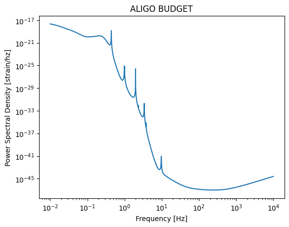
Getting the LIGO Sensitivity Curve

f_Hz = np.geomspace(1e-2, 1e4, 2000)
budget = gwinc.load_budget('aLIGO', freq=f_Hz)
trace_PSD = budget.run(freq=f_Hz).psd

plt.title("ALIGO BUDGET")
plt.loglog(f_Hz, trace_PSD)
plt.xlabel("Frequency [Hz]")
plt.ylabel("Power Spectral Density [strain/hz]")

Text(0, 0.5, 'Power Spectral Density [strain/hz]')

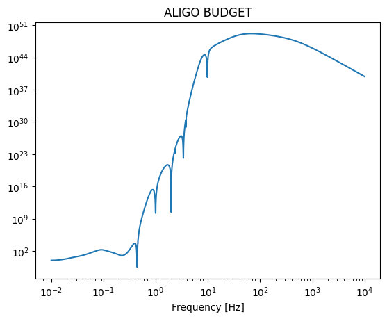
Lastly for this step we will combine the twu curves to make a FOM. we divide the BNS PSD by the LIGO Noise spectrum without the controls noise. From the paper: $$\mathrm{SNR}^2 = 4\int_{0}^{\infty} \frac{\left |h_\mathrm{gw}(f)\right |^2}{S_h(f)} df$$

where $S_h(f)$ is the noise spectrum of the detector. This can be written as:

$$ S_h(f) = S_{\mathrm{det}}(f) + |C(f)|^2 S_{\mathrm{p}}(f)$$

where $S_{\mathrm{det}}(f)$ is the detector noise spectrum without controls noise, $S_{\mathrm{p}}(f)$ is the control noise spectrum, and $C(f)$ is the coupling function from the controls noise in the control loop to DARM. By using the taylor series of A/(B+x) to linearize the integral. i.e.:

$$\frac{A}{B+x}=\frac{A}{B} - \frac{Ax}{B^2} + \frac{Ax^2}{B^3} - \frac{Ax^3}{B^4} + \frac{Ax^4}{B^5} - \frac{Ax^5}{B^6} + O(x^6)$$

taking the first two terms of the taylor series and applying it to the SNR equation we get:

$$\mathrm{SNR}^2 = 4\int_{0}^{\infty} \frac{\left | h_{\mathrm{signal}}(f)\right |^2}{S_{\mathrm{det}}(f)} \ df - 4\int_{0}^{\infty} \frac{\left |C\right |^2\left | h_{\mathrm{signal}}(f)\right |^2 }{S_{\mathrm{det}}(f)^2} S_{\mathrm{p}}(f) \ df$$

To get range we need to use the $\mathrm{SNR}$ not the $\mathrm{SNR}^2$ so we take the square root of the above equation which has a different linearization. as $A \rightarrow \infty$

$$\sqrt{A+B} = \sqrt{A} \sqrt{1+\frac{B}{A}} = \sqrt{A} (1+\frac{B}{2 \sqrt{A}})$$

from inspiral_range import inspiral_range as ir
linearization_PSD = trace_PSD**2
FOM_intgrand = ir.sensemon_range(f_Hz, psd=linearization_PSD, m1=1.4, m2=1.4, horizon=False, integrate=False, detection_snr=8)**2

f_Hz = np.geomspace(1e-2, 1e4, 2000)
budget = gwinc.load_budget('aLIGO', freq=f_Hz)
trace_PSD = budget.run(freq=f_Hz).psd

plt.title("ALIGO BUDGET")
plt.loglog(f_Hz, FOM_intgrand)
plt.xlabel("Frequency [Hz]")

Text(0.5, 0, 'Frequency [Hz]')

print(ir.sensemon_range(f_Hz, psd=linearization_PSD, m1=1.4, m2=1.4, horizon=False, integrate=True, detection_snr=8))
FOM_intgrand = ir.sensemon_range(f_Hz, psd=linearization_PSD, m1=1.4, m2=1.4, horizon=False, integrate=False, detection_snr=8)**2
print(np.trapezoid(FOM_intgrand, f_Hz)**0.5)

4.547336892714717e+25
4.547336892714716e+25

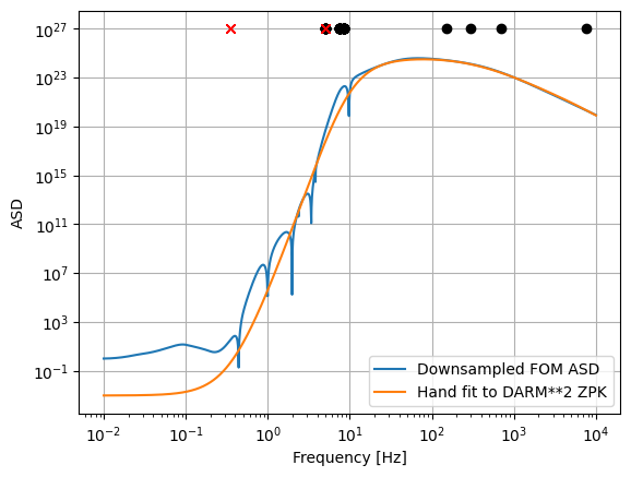
# Hand Fit the DARM**2 ZPK
shift_sq = 0.8
z_hand_sq = np.array([-0.07]*18) * 2 * np.pi * shift_sq
mp_sq = -0.75 -0.075j
mul_sq = 9
p_hand_sq = np.array([mp_sq]*mul_sq + [np.real(mp_sq)-np.imag(mp_sq)*1j]*mul_sq)*2 * 2 * np.pi * shift_sq
p_hand_sq = np.append(p_hand_sq, np.array([-150]*1 +[-300]*1 +[-700]*1 + [-7500]*1))
k_hand_sq = 1e36

##making steeper roll off
mp_sq = mp_sq * 2.25
p_hand_sq = np.append(p_hand_sq, np.array([mp_sq]*8 +[np.real(mp_sq)-np.imag(mp_sq)*1j]*8+ [-1]*8)* 2 * np.pi * shift_sq)
z_hand_sq = np.append(z_hand_sq, np.array([-1]*24)* 2 * np.pi * shift_sq)

#k_hand_sq = k_hand_sq *1e9

#plt.loglog(F_bug, Div_PSD**0.5, label = "Full FOM ASD")
plt.loglog(f_Hz, FOM_intgrand**0.5, label = "Downsampled FOM ASD")
#plt.loglog(F_Hz, abs(TF_all), label = 'ALL ZPK Fit Bary. (order {})'.format(results.order))
fq_plot = np.logspace(-2, 5, 10000)


hand_sys = SISO.zpk(z_hand_sq, p_hand_sq, k_hand_sq, convention='IIRrational')
#fr_hand = hand_sys.fresponse(f=fq_plot)
fr_hand = hand_sys.fresponse(f=f_Hz)

plt.loglog(-np.real(p_hand_sq), np.array([1e27]*len(p_hand_sq)), color='black', linestyle='', marker='o')
plt.loglog(-np.real(z_hand_sq), np.array([1e27]*len(z_hand_sq)), color='r', linestyle='', marker='x')
plt.loglog(*fr_hand.fplot_mag, label = 'Hand fit to DARM**2 ZPK')
plt.xlabel("Frequency [Hz]")
plt.ylabel("ASD")

plt.grid()
plt.legend()

#plt.savefig('FOM_BNS_fit.pdf', bbox_inches='tight')

/Users/Ian/miniconda3/envs/controls/lib/python3.10/site-packages/wield/control/SISO/zpk.py:164: NumericalWarning: StateSpace is large (>50 states), using reduced response fiducial auditing heuristics. TODO to make this smarter
  warnings.warn(f"StateSpace is large (>{self.N_MAX_FID} states), using reduced response fiducial auditing heuristics. TODO to make this smarter", util.NumericalWarning)

<matplotlib.legend.Legend at 0x12c900c40>

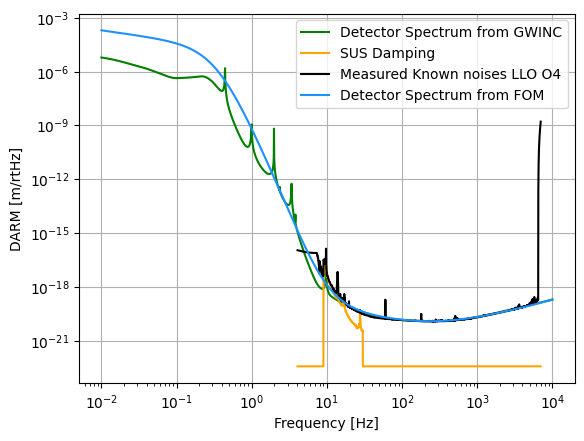
Next we calculate what this spectrum will look like from this FOM

LLO_O4_DARM = np.loadtxt('O4_data/L1_darm_measured.txt').T
LLO_O4_DARM_known = np.loadtxt('O4_data/L1_darm_known_measured.txt').T
LLO_O4_SUS_damping = np.loadtxt('O4_data/L1_sus_damping.txt').T

L_arm = 3995

BNS_range_inv = ir.sensemon_range(f_Hz, psd=np.ones_like(f_Hz), m1=1.4, m2=1.4, horizon=False, integrate=False, detection_snr=8)**2
det_PSD_from_FOM = ((BNS_range_inv)/fr_hand.mag**2)**0.5
plt.loglog(f_Hz, trace_PSD**0.5*L_arm , label = 'Detector Spectrum from GWINC', color='green')
# plt.loglog(LLO_O4_DARM[0], LLO_O4_DARM[1]*L_arm , label = 'Measured DARM LLO O4', color='red')
plt.loglog(LLO_O4_SUS_damping[0], LLO_O4_SUS_damping[1]*L_arm , label = 'SUS Damping', color='orange')
plt.loglog(LLO_O4_DARM_known[0], LLO_O4_DARM_known[1]*L_arm , label = 'Measured Known noises LLO O4', color='black')
plt.loglog(f_Hz, det_PSD_from_FOM**0.5*L_arm , label = 'Detector Spectrum from FOM', color='dodgerblue')
plt.xlabel("Frequency [Hz]")
plt.ylabel("DARM [m/rtHz]")

# plt.xlim([6, 10000])
# plt.ylim([1e-20, 1e-15])

plt.grid()
plt.legend()

<matplotlib.legend.Legend at 0x169ca1000>

Now we will save our result so it can be loaded by the make full system example file

out_z = z_hand_sq
out_p = p_hand_sq
out_k = k_hand_sq

pre_save_sys = SISO.zpk(out_z, out_p, out_k, convention='IIRrational')
from wield.utilities.mpl import mplfigB
plotting_omega = np.logspace(-2, 4, 1000)
plt.close()
axB = mplfigB(Nrows = 2)
fr = pre_save_sys.fresponse(f=plotting_omega)
axB.ax0.loglog(*fr.fplot_mag, label='test')
axB.ax1.semilogx(*fr.fplot_deg225, label='test')


sys_save = SISO.zpk(out_z, out_p, out_k, convention='IIRrational')
assert(ssutil.isStable(sys_save))
zpk_dict = {
            'z' : [str(zero) for zero in np.asarray(tuple(sys_save.z)).tolist()],
            'p' : [str(pole) for pole in np.asarray(tuple(sys_save.p)).tolist()],
            'k' : float(sys_save.k)
            }

#save('BNS_FOM_IR.yml', zpk_dict) #Uncomment to save the ZPK

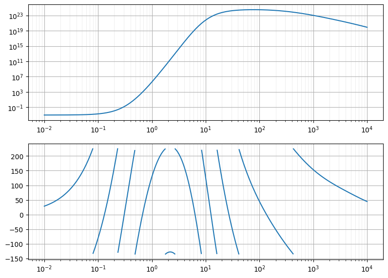
Now it is saved. To open it use the following code

with open('BNS_FOM.yml', 'r') as file:
    filt_dict = yaml.safe_load(file)
p = np.array(filt_dict['p'], dtype=np.complex128)
z = np.array(filt_dict['z'], dtype=np.complex128)
k = np.float64(filt_dict['k'])
print(type(k))
print(len(z))
print(len(p))

<class 'numpy.float64'>
49
52