Fitting Data and Making FOMs

Here I will go through an example of how to fit data to a transfer function. Later this TF will be used to make a full system model.

First imports:

%load_ext autoreload
%autoreload 2
import numpy as np
import matplotlib.pyplot as plt
import control
import scipy.signal as signal
from scipy import interpolate
import scipy.linalg
from scipy.stats import gmean
import gwinc
import yaml
from wield.iirrational.v2 import data2filter
from wield.control.AAA import tfAAA
from wield.utilities.file_io import load, save
from wield.control.ss_bare.ss import BareStateSpace
from scipy.signal import cheby2
from wield.control import SISO
from buzz import ssutil
from physunits import m, s, kg, Hz
from scipy.constants import c, G

Next we will define a function to grab the BNS waveform

# from https://github.com/wield/wield-control/blob/main/src/wield/control/AAA/test/test_AAA_present.py
def gen_waveform(**params):
    """Generate frequency-domain inspiral waveform

    Returns a tuple of (freq, h_plus^tilde, h_cross^tilde).

    The waveform is generated with the lalsimulation
    SimInspiralChooseFDWaveform() function.  Keyword arguments are
    used to update the default waveform parameters (see DEFAULT_PARAMS
    macro).  The mass parameters ('m1' and 'm2') should be specified
    in solar masses and the 'distance' parameter should be specified
    in parsecs**.  Waveform approximants may be given as string names
    (see `lalsimulation` documentation for more info).

    For example, to generate a 20/20 Msolar BBH waveform:

    >>> hp,hc = waveform.gen_waveform('m1'=20, 'm2'=20)

    **NOTE: The requirement that masses be specified in solar masses
    and distances in parsecs is different than that of the underlying
    lalsimulation method which expects mass and distance parameters to
    be in SI units.

    """
    import lalsimulation
    from inspiral_range import waveform
    from inspiral_range import const

    iparams = dict(waveform.DEFAULT_PARAMS)
    iparams.update(**params)

    # convert to SI units
    iparams["distance"] *= const.PC_SI
    iparams["m1"] *= const.MSUN_SI
    iparams["m2"] *= const.MSUN_SI
    iparams["approximant"] = lalsimulation.SimInspiralGetApproximantFromString(
        iparams["approximant"]
    )

    m = iparams["m1"] + iparams["m2"]

    # calculate delta F based on frequency of inner-most stable
    # circular orbit ("fisco")
    fisco = (const.c ** 3) / (const.G * (6 ** 1.5) * 2 * np.pi * m)
    df = 2 ** (np.max([np.floor(np.log(fisco / 4096) / np.log(2)), -6]))

    # FIXME: are these limits reasonable?
    if iparams["deltaF"] is None:
        iparams["deltaF"] = df
    # iparams['f_min'] = 0.1
    # iparams['f_max'] = 10000

    hp, hc = lalsimulation.SimInspiralChooseFDWaveform(**iparams)
    
    freq = hp.f0 + np.arange(len(hp.data.data)) * hp.deltaF

    print("f0", hp.f0)
    select = abs(hp.data.data) > 0

    return freq[select], hp.data.data[select], hc.data.data[select]

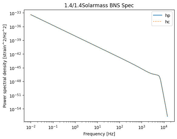
Next we will define the parameters of our BNS model and plot its PSD

params = dict()
params["m1"] = 1.4
params["m2"] = 1.4
# rest of params from first BNS detection see https://journals.aps.org/prl/pdf/10.1103/PhysRevLett.119.161101
params["f_min"] = 0.01
params["f_max"] = 1000000
params["deltaF"] = 0.01
params["distance"] = 1e6
F_Hz, hp, hc = gen_waveform(**params) # assuming that this is giving an ASD I.M. Jan 2024

BNS_intrp = interpolate.interp1d(F_Hz, abs(hp)**2) ## we add interpolation to put all of our data with the same FQ spacing

print("F_Hz max", max(F_Hz))

plt.loglog(F_Hz, abs(hp)**2, label = "hp")
plt.loglog(F_Hz, abs(hc)**2, linestyle = ":", label = "hc")
plt.title(str(params["m1"]) +"/"+str(params["m1"])+ "Solarmass BNS Spec")
plt.xlabel("Frequency [Hz]")
plt.ylabel("Power spectral density [strain^2/Hz^2]")
plt.legend()
plt.show()

f0 0.0
F_Hz max 14501.800000000001

# # compare the waveform with part of equation 3 from https://arxiv.org/abs/1709.08079
m1 = (params["m1"] * 1.988416e30) * kg
m2 = (params["m2"] * 1.988416e30) * kg
chirp_mass = (m1*m2)**(3/5)/(m1+m2)**(1/5)
print('chirpmass: \t', chirp_mass, ' kg\n\t\t', chirp_mass/1.988416e30, ' solar masses')


# N = kg* m/(s**2)
# c = c * m/s
# G = G * N * m**2 / (kg**2)
# F_Hz = F_Hz * Hz
# eq3 = ((5/24)**0.5 * c * ( G * chirp_mass * (c**-3))**(5/6)* 1/(np.pi**(2/3)))**2 * F_Hz**(-7/3)
# m2Mpc = 1/3.086e22
# eq3_Mpc = eq3 * m2Mpc

# print("eq3[0]", eq3[0])
# print("eq3_Mpc[0]", eq3_Mpc[0])

# print("BNS hp[0]", abs(hp[0])**2)

# plt.loglog(F_Hz, eq3_Mpc, label="eq3")
# plt.loglog(F_Hz, abs(hp)**2, label="BNS Strain from LAL Simulation")
# plt.title(str(params["m1"]) +"/"+str(params["m1"])+ "Solarmass BNS Spec")
# plt.xlabel("Frequency [Hz]")
# plt.ylabel("Power spectral density [strain^2/Hz^2]")
# plt.legend()
# plt.show()

chirpmass: 	 2.423423336413827e+30  kg
		 1.2187707886145691  solar masses

Getting the LIGO Sensitivity Curve

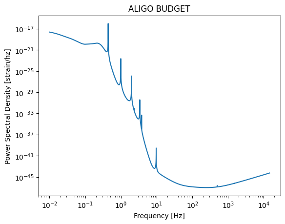
Now I must multiply this by the GWINC curve to get our final FOM

F_bug = np.logspace(np.log10(min(F_Hz)), np.log10(max(F_Hz)-1), 10000)
budget = gwinc.load_budget('aLIGO', freq=F_bug)
trace = budget.run(freq=F_bug)

plt.title("ALIGO BUDGET")
plt.loglog(F_bug, trace.psd)
plt.xlabel("Frequency [Hz]")
plt.ylabel("Power Spectral Density [strain/hz]")
# plt.xlim([6, max(F_Hz)])
# plt.ylim([1e-20, 1e-17])

Text(0, 0.5, 'Power Spectral Density [strain/hz]')

prefactor = (2*(5/96)**0.5 * c * ( G * chirp_mass * (c**3))**(5/6) * 1/(np.pi**(-2/3))* 2 / 2.26)**2 
I7 = np.trapz(F_bug**(-7/3)/trace.psd, F_bug)
eq3 = prefactor * I7**0.5
print("eq3: ", eq3/3.086e22, ' Mpc')

eq3:  4.8671221455438923e+92  Mpc

/var/folders/mg/zt3ys6wx6dv2lp4fp2v08nn80000gn/T/ipykernel_49986/2399436929.py:2: DeprecationWarning: `trapz` is deprecated. Use `trapezoid` instead, or one of the numerical integration functions in `scipy.integrate`.
  I7 = np.trapz(F_bug**(-7/3)/trace.psd, F_bug)

from inspiral_range import inspiral_range as ir
from inspiral_range import waveform
from inspiral_range import const

DETECTION_SNR = 8.0
def ian_sensemon_range(freq, m1=1.4, m2=1.4, horizon=False, integrate=False, detection_snr=DETECTION_SNR):
    """Detector inspiral range from closed form expression

    Masses `m1` and `m2` should be specified in solar masses (default:
    m1=m2=1.4).  If the `horizon` keyword is specified the "horizon"
    range will be returned, which differs from the angle-averaged
    range by ~2.26.

    @returns distance in Mpc as a float

    """
    if horizon:
        theta = 4
    else:
        theta = 1.77
    theta /= 1e6 * const.PC_SI
    M_chirp = waveform.M_chirp(m1, m2) * const.MSUN_SI

    i73 = freq ** (-7/3)
    val = theta / detection_snr \
        * waveform.habs_nsp_prefactor(M_chirp) \
        * np.sqrt(i73) / 2

    return val

irdata = ian_sensemon_range(F_bug, integrate=False, horizon=True)**2

range_ir = ir.sensemon_range(F_bug, psd=trace.psd, m1=1.4, m2=1.4, horizon=False, integrate=True, detection_snr=DETECTION_SNR)
print("range: ", range_ir)

#np.savetxt('FBNS_Current_range.txt', [range])

BNS_PSD = BNS_intrp(F_bug)
IR_interp = interpolate.interp1d(F_bug, irdata)

midpoint = len(F_bug)//2
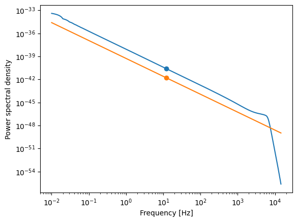
print('relative difference: ', BNS_PSD[midpoint]/irdata[midpoint])


plt.loglog(F_bug, BNS_PSD)
plt.loglog(F_bug, irdata)
plt.scatter(F_bug[midpoint], BNS_PSD[midpoint])
plt.scatter(F_bug[midpoint], irdata[midpoint])
plt.xlabel("Frequency [Hz]")
plt.ylabel("Power spectral density");

range:  194.97356835627136
relative difference:  15.834426262915697

Choose which inspiral waveform PSD to use

#BNS_PSD = BNS_intrp(F_bug) # us the custom inspiral equatin from LAL
BNS_PSD = IR_interp(F_bug) # use the inspiral range aproximation and calibration 

Now I will put the BNS waveform in the Fq space of the GWINC curve

print("BNS_PSD", BNS_PSD)
print("irdata", irdata)
plt.loglog(F_bug, BNS_PSD)
plt.xlabel("Frequency [Hz]")
plt.ylabel("Power spectral density")

BNS_PSD [2.45847170e-35 2.45034599e-35 2.44224714e-35 ... 1.03982336e-49
 1.03638655e-49 1.03296110e-49]
irdata [2.45847170e-35 2.45034599e-35 2.44224714e-35 ... 1.03982336e-49
 1.03638655e-49 1.03296110e-49]

Text(0, 0.5, 'Power spectral density')

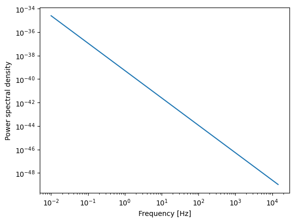
Lastly for this step we will combine the twu curves to make a FOM. we divide the BNS PSD by the LIGO Noise spectrum without the controls noise. From the paper: $$\mathrm{SNR}^2 = 4\int_{0}^{\infty} \frac{\left |h_\mathrm{gw}(f)\right |^2}{S_h(f)} df$$

where $S_h(f)$ is the noise spectrum of the detector. This can be written as:

$$ S_h(f) = S_{\mathrm{det}}(f) + |C(f)|^2 S_{\mathrm{p}}(f)$$

where $S_{\mathrm{det}}(f)$ is the detector noise spectrum without controls noise, $S_{\mathrm{p}}(f)$ is the control noise spectrum, and $C(f)$ is the coupling function from the controls noise in the control loop to DARM. By using the taylor series of A/(B+x) to linearize the integral. i.e.:

$$\frac{A}{B+x}=\frac{A}{B} - \frac{Ax}{B^2} + \frac{Ax^2}{B^3} - \frac{Ax^3}{B^4} + \frac{Ax^4}{B^5} - \frac{Ax^5}{B^6} + O(x^6)$$

taking the first two terms of the taylor series and applying it to the SNR equation we get:

$$\mathrm{SNR}^2 = 4\int_{0}^{\infty} \frac{\left | h_{\mathrm{signal}}(f)\right |^2}{S_{\mathrm{det}}(f)} \ df - 4\int_{0}^{\infty} \frac{\left |C\right |^2\left | h_{\mathrm{signal}}(f)\right |^2 }{S_{\mathrm{det}}(f)^2} S_{\mathrm{p}}(f) \ df$$

To get range we need to use the $\mathrm{SNR}$ not the $\mathrm{SNR}^2$ so we take the square root of the above equation which has a different linearization. as $A \rightarrow \infty$

$$\sqrt{A+B} = \sqrt{A} \sqrt{1+\frac{B}{A}} = \sqrt{A} (1+\frac{B}{2 \sqrt{A}})$$

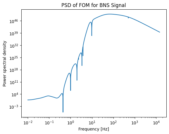
Div_PSD = BNS_PSD / (trace.psd)**2 # divide the BNS PSD by the aLIGO noise psd squared. this will give a PSD of LIGO's sensitivity to a BNS signal
#Div_PSD = Div_PSD * 4000**2 # to put it in units of displacement
F_Div = F_bug
plt.loglog(F_Div, Div_PSD)
plt.xlabel("Frequency [Hz]")
plt.ylabel("Power spectral density")
plt.title("PSD of FOM for BNS Signal")

Text(0.5, 1.0, 'PSD of FOM for BNS Signal')

Fitting the Data to a Transfer Function

First we will Define a function to reduce the number of points to fit to

# edited from https://git.ligo.org/wield/wield-ligo-mcculler/-/blob/main/src/wield/LIGO/mcculler/filter_cavity/test_FC1_SUSPOINT_fits.py
def reduce(F_Hz, PSD):
    F_groups = np.logspace(-2, 4, 50) # originally 200 length
    F_groups = np.geomspace(min(F_Hz), max(F_Hz), 50) # originally 200 length
    
    idx_groups = np.searchsorted(F_Hz, F_groups)
    idx_pairs = list(zip(idx_groups[:-1], idx_groups[1:]))

    lPSDs_min = []
    lPSDs_max = []
    lPSDs_med = []
    lPSDs_mean = []
    lF_Hz = []
    for idx1, idx2 in idx_pairs:
        if idx1 == idx2:
            continue
        lPSDs_max.append(
            np.nanmax(PSD[idx1:idx2])
        )
        lPSDs_med.append(
            np.nanmedian(PSD[idx1:idx2])
        )
        lPSDs_min.append(
            np.nanmin(PSD[idx1:idx2])
        )
        lPSDs_mean.append(
            np.nanmean(PSD[idx1:idx2])
        )
        lF_Hz.append(np.mean(F_Hz[idx1:idx2]))

    return np.asarray(lF_Hz), np.asarray(lPSDs_min), np.asarray(lPSDs_med), np.asarray(lPSDs_max), np.asarray(lPSDs_mean)

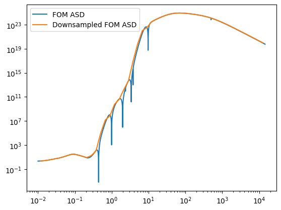
Now we will reduce the LIGO sensitivity curve and its reduced form

F_FOM_dwn, PSD_min, PSD_med, PSD_max, PSD_mean = reduce(F_bug, Div_PSD)
FOM_PSD = PSD_mean
# The current form of FOM_PSD is the ASD
FOM_ASD = FOM_PSD**0.5

plt.loglog(F_bug, Div_PSD**0.5, label = 'FOM ASD')
plt.loglog(F_FOM_dwn, FOM_ASD, label = 'Downsampled FOM ASD')
plt.legend()

<matplotlib.legend.Legend at 0x16ca8e8c0>

Now we will define some functions to work with these transfer functions

def FBNSsimpSS(gain=1, return_name=False, lo_ord=4):
    if return_name:
        name = "FOM BNS Simple"
        return name
    F_Fq_lo = 10 * 2 * np.pi
    F_Fq_hi = 120 * 2 * np.pi
    hp_order = lo_ord
    lp_order = 2
    F_p = []
    F_z = []
    for ord in range(hp_order):
        F_p.append(-F_Fq_lo + 0*1j*F_Fq_lo)
        F_p.append(-F_Fq_lo - 0*1j*F_Fq_lo)
        F_z.append(0)
        F_z.append(0)

    for ord in range(lp_order):
        F_p.append(-F_Fq_hi)
    F_k = 1
    c_zpk = cheby2(8, 170, 1.25*2*np.pi, btype='high', analog=True, output='zpk')
    F_z.extend(c_zpk[0])
    F_p.extend(c_zpk[1])
    F_k *= c_zpk[2]

    ian_lfq = -0.7
    ian_lfq2 = 2
    ian_lfq3 = 0.5
    F_z.append(0)
    F_p.append(ian_lfq)
    F_z.append(0)
    F_p.append(ian_lfq)

    F_z.append(ian_lfq3)
    F_z.append(ian_lfq3)
    F_p.append(ian_lfq2)
    F_p.append(ian_lfq2)
    
    F_p = F_p
    F_z = F_z

    #F_mod = ws_tf2ss(F_z, F_p, F_k)
    #F_mod = ssutil.normalize_gain(F_mod) * gain 
    #F_iod = {"FBNS.in": 0, "FBNS.out": 0}
    F_mod = SISO.zpk(F_z, F_p, F_k, angular=True, fiducial_rtol=1e-5, fiducial_atol=1e-10)
    F_mod = F_mod * F_mod
    F_mod = F_mod.asSS
    F_mod = F_mod / abs(F_mod.asSS.Linf_norm()[0]) 


    F_mod = F_mod * gain
    F_mod.balance_and_truncate()

    #F = ssutil.wieldSS(F_mod, F_iod)
    
    return F_mod.mimo("FBNS.in", "FBNS.out")

plt.loglog(F_bug, Div_PSD**0.5, label = 'FOM ASD')
plt.loglog(F_FOM_dwn, FOM_ASD, label = 'Downsampled FOM ASD')
mag, phase, omega = control.bode(FBNSsimpSS(gain=4 * 100**2).mod, Hz=False, plot=False, omega=F_FOM_dwn*2*np.pi, label = "BNS Simple")
#plt.loglog(omega/(2*np.pi), mag, label="BNS Simple")
plt.legend()

/Users/Ian/miniconda3/envs/controls/lib/python3.10/site-packages/wield/control/SISO/zpk.py:164: NumericalWarning: StateSpace is large (>50 states), using reduced response fiducial auditing heuristics. TODO to make this smarter
  warnings.warn(f"StateSpace is large (>{self.N_MAX_FID} states), using reduced response fiducial auditing heuristics. TODO to make this smarter", util.NumericalWarning)
/Users/Ian/miniconda3/envs/controls/lib/python3.10/site-packages/slycot/exceptions.py:241: SlycotResultWarning: 
The selected order 44 is greater
than `nsmin`, the sum of the order of the
0-unstable part and the order of a minimal
realization of the 0-stable part of the given
system. The resulting `nr`  is set to `nsmin` = 33
  warn(globals()[warning](fmessage, iwarn, info))

<matplotlib.legend.Legend at 0x14f5f00a0>

from scipy.signal import cheby2
from wield.control import SISO

def FBNSsimpSS(gain=1, return_name=False, lo_ord=4, return_scale=False):
    if return_name:
        name = "FOM BNS Simple"
        return name
    
    F_Fq_lo = 40 * 2 * np.pi
    # aggressive version
    # F_Fq_lo = 30 * 2 * np.pi
    F_Fq_hi = 300 * 2 * np.pi
    hp_order = 1 #lo_ord
    lp_order = 2
    F_p = []
    F_z = []
    for ord in range(hp_order):
        F_p.append(-F_Fq_lo + 0*1j*F_Fq_lo)
        F_p.append(-F_Fq_lo - 0*1j*F_Fq_lo)
        F_z.append(0)
        F_z.append(0)
    for ord in range(lp_order):
        F_p.append(-F_Fq_hi)
    F_k = gain * 1.5e19
    c_zpk = cheby2(8, 160, 4*2*np.pi, btype='high', analog=True, output='zpk')
    # aggressive version
    # c_zpk = cheby2(8, 120, 4*2*np.pi, btype='high', analog=True, output='zpk')
    F_z.extend(c_zpk[0])
    F_p.extend(c_zpk[1])
    F_k *= c_zpk[2]
    
    F = SISO.zpk(F_z, F_p, F_k)
    return F*F
sys_FBNS_simp = FBNSsimpSS()

zpk_dict = {
            'z' : [str(zero) for zero in np.asarray(tuple(sys_FBNS_simp.z)).tolist()],
            'p' : [str(pole) for pole in np.asarray(tuple(sys_FBNS_simp.p)).tolist()],
            'k' : float(sys_FBNS_simp.k)
            }

save('FBNSsimp_FOM.yml', zpk_dict)

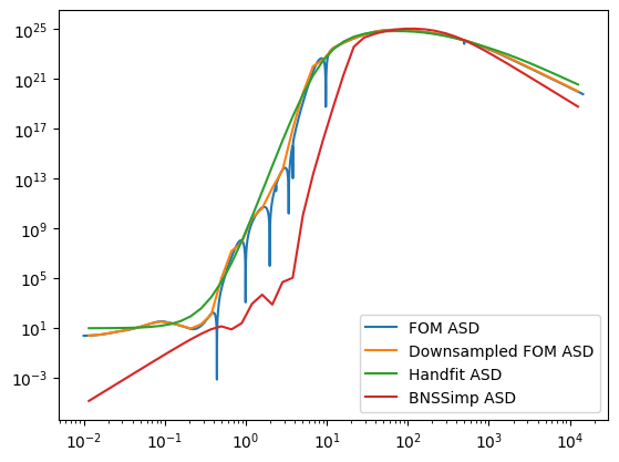
with open('BNS_FOM_handfit.yml', 'r') as file:
    filt_dict = yaml.safe_load(file)
p_hand = np.array(filt_dict['p'], dtype=np.complex128)
z_hand = np.array(filt_dict['z'], dtype=np.complex128)
k_hand = np.float64(filt_dict['k'])

hand_zpk = SISO.zpk(z_hand, p_hand, k_hand)
hand_xfr = hand_zpk.fresponse(f=F_FOM_dwn)
BNSsimp_xfr = sys_FBNS_simp.fresponse(f=F_FOM_dwn)

plt.loglog(F_bug, Div_PSD**0.5, label = 'FOM ASD')
plt.loglog(F_FOM_dwn, FOM_ASD, label = 'Downsampled FOM ASD')
plt.loglog(F_FOM_dwn, hand_xfr.mag, label = 'Handfit ASD')
plt.loglog(F_FOM_dwn, BNSsimp_xfr.mag, label = 'BNSSimp ASD')
plt.legend()

<matplotlib.legend.Legend at 0x3262ada50>

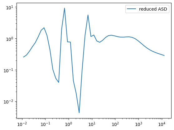
# Divide the FOM ASD by the hand fit to get the reduced ASD
reduced_ASD = FOM_ASD/hand_xfr.mag

plt.loglog(F_FOM_dwn, reduced_ASD, label = 'reduced ASD')
plt.legend()

<matplotlib.legend.Legend at 0x3265c1300>

Now we form a guess of the TF

#results = tfAAA(F_Hz=F_FOM_dwn, xfer=FOM_ASD)
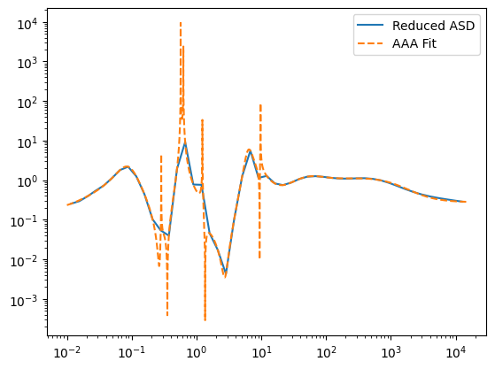
results = tfAAA(F_Hz=F_FOM_dwn, xfer=reduced_ASD)

Now we play with the poles and zeros to get a good fit

#print("poles", results.poles)
#print("zeros", results.zeros)
#print("gain", results.gain)

all_z = results.zeros
all_p = results.poles
k = results.gain

for i in range(0, len(all_z)):
    if all_z[i] >= 0:
        all_z[i] = -all_z[i]
        
for i in range(0, len(all_p)):
    if all_p[i] >= 0:
        all_p[i] = -all_p[i]

AAA_zpk = SISO.zpk(all_z, all_p, k, angular=False, fiducial_rtol=1e-5, fiducial_atol=1e-10)
recalibrated_zpk =  hand_zpk * AAA_zpk 
# recalibrated_zpk =  AAA_zpk 
print(recalibrated_zpk.zeros)

2π·[-0.3958406743523140, -0.3958406743523140, -0.3958406743523140,
 -0.3958406743523140, -0.3958406743523140, -0.3958406743523140,
 -0.3958406743523140, -0.3958406743523140, -0.3958406743523140,
 -0.3958406743523140, -0.3958406743523140, -0.3958406743523140,
 -0.3958406743523140, -0.3958406743523140, -0.3958406743523140,
 -0.3958406743523140, -0.3958406743523140, -0.3958406743523140,
 -0.01203291268450893, -0.01203291245508902, -2.972731813094795e-10,
 -0.04867452063486528, -0.04867452070907659, -1.998523750481311,
 -1.998523750486431, -2665.214389252330, -2665.214389239281,
 -92.39465985988777     ± 57.24588444085094j,
 -92.39465986028216     ± 57.24588444036313j,
 -3.274971594925781e-14 ± 9.399266058512616j,
 -2.736440429942560e-13 ± 1.357591960953234j,
 -0.01049742774282587   ± 0.2673257560166767j,
 -0.01049742774343546   ± 0.2673257560021555j,
 -1.092192520377326e-12 ± 0.3543630287392169j,
 -0.2711283246749082    ± 2.729288190523091j,
 -0.2711283246761620    ± 2.729288190522066j,
 -13.03329719065969     ± 14.32232176510654j,
 -13.03329719064406     ± 14.32232176511557j]

plt.loglog(F_FOM_dwn, reduced_ASD, label = 'Reduced ASD')
plt.loglog(F_bug, AAA_zpk.fresponse(f=F_bug).mag, label = 'AAA Fit', linestyle = '--')
plt.legend()

<matplotlib.legend.Legend at 0x3307ee1d0>

# Get the ZPK and the minreal ZPK for all poles and zeros
B_res_all = control.zpk(all_z, all_p, k)
B_res_all_minreal = control.minreal(B_res_all)
minreal_all_z, minreal_all_p, minreal_all_k = signal.tf2zpk(B_res_all_minreal.num[0][0], B_res_all_minreal.den[0][0])

# Get only the real poles and zeros
z = [lz for lz in all_z if lz.real < 0]
p = [lp for lp in all_p if lp.real < 0]

# Get the ZPK for the real poles and zeros and the minreal ZPK for only the real poles and zeros
B_res = control.zpk(z, p, k)
B_res_minreal = control.minreal(B_res)
minreal_z, minreal_p, minreal_k = signal.tf2zpk(B_res_minreal.num[0][0], B_res_minreal.den[0][0])

0 states have been removed from the model
0 states have been removed from the model

/Users/Ian/miniconda3/envs/controls/lib/python3.10/site-packages/control/xferfcn.py:1047: ComplexWarning: Casting complex values to real discards the imaginary part
  den[j, :maxindex+1] = poly(poles[j])
/Users/Ian/miniconda3/envs/controls/lib/python3.10/site-packages/control/xferfcn.py:1077: ComplexWarning: Casting complex values to real discards the imaginary part
  num[i, j, maxindex+1-len(numpoly):maxindex+1] = numpoly

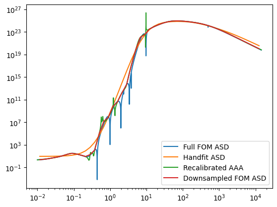
Now we will plot our guess and our othe tfs

_, TF_all = scipy.signal.freqs_zpk(all_z, all_p, k, worN = F_Hz)
_, TF_minreal = scipy.signal.freqs_zpk(minreal_all_z, minreal_all_p, minreal_all_k, worN = F_Hz)

recalibrated_zpk_xfr = recalibrated_zpk.fresponse(f=F_Hz)

plt.loglog(F_bug, Div_PSD**0.5, label = 'Full FOM ASD')
plt.loglog(F_FOM_dwn, hand_xfr.mag, label = 'Handfit ASD')
plt.loglog(F_Hz, recalibrated_zpk_xfr.mag, label = 'Recalibrated AAA')
plt.loglog(F_FOM_dwn, FOM_ASD, label = 'Downsampled FOM ASD')
#plt.loglog(F_Hz, abs(TF_all), label = 'ALL ZPK Fit Bary. (order {})'.format(results.order))
#plt.loglog(F_Hz, abs(TF_minreal), label = 'Minreal ALL ZPK Fit Bary.', linestyle = '--')
plt.legend()

<matplotlib.legend.Legend at 0x330b8f790>

Now we fit for the poles and zeros

snr = np.ones_like(F_FOM_dwn)
snr[:-1] = (F_FOM_dwn[1:] - F_FOM_dwn[:-1])**-0.001
from wield.iirrational import fitters_ZPK

all_z = (np.array(recalibrated_zpk.zeros))
all_p = (np.array(recalibrated_zpk.poles))
k = float(recalibrated_zpk.k)

z_iir = tuple(np.array(all_z) / (np.pi * 2))
p_iir = tuple(np.array(all_p) / (np.pi * 2))
print(z_iir)
print(p_iir)

iir_results = data2filter(
    F_Hz=F_FOM_dwn,
    xfer=FOM_ASD,
    #xfer=reduced_ASD,
    mode='reduce',
    zeros=z_iir, 
    poles=p_iir,
    gain=k * (2*np.pi)**(len(z_iir) - len(p_iir)),
    SNR_phase_rel=0,
    SNR=snr,
    #relative_degree=-4,
    # resavg_RthreshOrdDn=1.01,
    baseline_only=True,
    #coding_map=fitters_ZPK.codings_s.coding_maps.RI
    # trust_SNR = True,
)
print("C", iir_results.fit_aid._fitters[0].fitter.poles.fullplane)
print(tuple(np.array(all_p) / (np.pi * 2)))

(np.float64(-0.395840674352314), np.float64(-0.395840674352314), np.float64(-0.395840674352314), np.float64(-0.395840674352314), np.float64(-0.395840674352314), np.float64(-0.395840674352314), np.float64(-0.395840674352314), np.float64(-0.395840674352314), np.float64(-0.395840674352314), np.float64(-0.395840674352314), np.float64(-0.395840674352314), np.float64(-0.395840674352314), np.float64(-0.395840674352314), np.float64(-0.395840674352314), np.float64(-0.395840674352314), np.float64(-0.395840674352314), np.float64(-0.395840674352314), np.float64(-0.395840674352314), np.float64(-0.012032912684508928), np.float64(-0.01203291245508902), np.float64(-2.972731813094795e-10), np.float64(-0.048674520634865284), np.float64(-0.048674520709076595), np.float64(-1.9985237504813107), np.float64(-1.9985237504864306), np.float64(-2665.21438925233), np.float64(-2665.2143892392814), np.complex128(-92.39465985988777+57.245884440850936j), np.complex128(-92.39465985988777-57.245884440850936j), np.complex128(-92.39465986028216+57.24588444036313j), np.complex128(-92.39465986028216-57.24588444036313j), np.complex128(-3.274971594925781e-14+9.399266058512616j), np.complex128(-3.274971594925781e-14-9.399266058512616j), np.complex128(-2.73644042994256e-13+1.357591960953234j), np.complex128(-2.73644042994256e-13-1.357591960953234j), np.complex128(-0.010497427742825865+0.26732575601667674j), np.complex128(-0.010497427742825865-0.26732575601667674j), np.complex128(-0.010497427743435463+0.26732575600215547j), np.complex128(-0.010497427743435463-0.26732575600215547j), np.complex128(-1.0921925203773264e-12+0.35436302873921693j), np.complex128(-1.0921925203773264e-12-0.35436302873921693j), np.complex128(-0.2711283246749082+2.7292881905230915j), np.complex128(-0.2711283246749082-2.7292881905230915j), np.complex128(-0.271128324676162+2.729288190522066j), np.complex128(-0.271128324676162-2.729288190522066j), np.complex128(-13.033297190659693+14.322321765106544j), np.complex128(-13.033297190659693-14.322321765106544j), np.complex128(-13.033297190644062+14.322321765115568j), np.complex128(-13.033297190644062-14.322321765115568j))
(np.float64(-200.0), np.float64(-200.0), np.float64(-1999.9999999999998), np.float64(-0.02007827991778461), np.float64(-0.020078279659776748), np.float64(-2.580708621122238e-10), np.float64(-15.278039002751779), np.float64(-15.27803900294391), np.float64(-37.5875499182891), np.float64(-37.58754992011324), np.float64(-1270.3160778915844), np.float64(-1270.3160778760625), np.complex128(-8.482300164692441+0.8482300164692441j), np.complex128(-8.482300164692441-0.8482300164692441j), np.complex128(-8.482300164692441+0.8482300164692441j), np.complex128(-8.482300164692441-0.8482300164692441j), np.complex128(-8.482300164692441+0.8482300164692441j), np.complex128(-8.482300164692441-0.8482300164692441j), np.complex128(-8.482300164692441+0.8482300164692441j), np.complex128(-8.482300164692441-0.8482300164692441j), np.complex128(-8.482300164692441+0.8482300164692441j), np.complex128(-8.482300164692441-0.8482300164692441j), np.complex128(-8.482300164692441+0.8482300164692441j), np.complex128(-8.482300164692441-0.8482300164692441j), np.complex128(-8.482300164692441+0.8482300164692441j), np.complex128(-8.482300164692441-0.8482300164692441j), np.complex128(-8.482300164692441+0.8482300164692441j), np.complex128(-8.482300164692441-0.8482300164692441j), np.complex128(-8.482300164692441+0.8482300164692441j), np.complex128(-8.482300164692441-0.8482300164692441j), np.complex128(-86.35143298229573+19.216867768387107j), np.complex128(-86.35143298229573-19.216867768387107j), np.complex128(-86.35143298333351+19.216867758926814j), np.complex128(-86.35143298333351-19.216867758926814j), np.complex128(-7.184546295609813e-13+9.719862477185815j), np.complex128(-7.184546295609813e-13-9.719862477185815j), np.complex128(-1.835561875225273e-13+1.2313225699476558j), np.complex128(-1.835561875225273e-13-1.2313225699476558j), np.complex128(-1.0967543329481134e-12+0.2850867195563693j), np.complex128(-1.0967543329481134e-12-0.2850867195563693j), np.complex128(-0.03919349729548207+0.08045695915767265j), np.complex128(-0.03919349729548207-0.08045695915767265j), np.complex128(-0.03919349729706598+0.0804569591557125j), np.complex128(-0.03919349729706598-0.0804569591557125j), np.complex128(-1.0663904270747737e-12+0.5688213957405965j), np.complex128(-1.0663904270747737e-12-0.5688213957405965j), np.complex128(-1.078838929878826e-12+0.6261479514724254j), np.complex128(-1.078838929878826e-12-0.6261479514724254j), np.complex128(-1.0344028607168105+6.179659433092568j), np.complex128(-1.0344028607168105-6.179659433092568j), np.complex128(-1.0344028607159552+6.179659433094185j), np.complex128(-1.0344028607159552-6.179659433094185j))
TEE_LOGFILE None
A [-2.00000000e+02 +0.j         -2.00000000e+02 +0.j
 -2.00000000e+03 +0.j         -2.00782799e-02 +0.j
 -2.00782797e-02 +0.j         -2.58070862e-10 +0.j
 -1.52780390e+01 +0.j         -1.52780390e+01 +0.j
 -3.75875499e+01 +0.j         -3.75875499e+01 +0.j
 -1.27031608e+03 +0.j         -1.27031608e+03 +0.j
 -8.48230016e+00 +0.84823002j -8.48230016e+00 -0.84823002j
 -8.63514330e+01+19.21686777j -8.63514330e+01-19.21686777j
 -8.63514330e+01+19.21686776j -8.63514330e+01-19.21686776j
 -7.18454630e-13 +9.71986248j -7.18454630e-13 -9.71986248j
 -1.83556188e-13 +1.23132257j -1.83556188e-13 -1.23132257j
 -1.09675433e-12 +0.28508672j -1.09675433e-12 -0.28508672j
 -3.91934973e-02 +0.08045696j -3.91934973e-02 -0.08045696j
 -3.91934973e-02 +0.08045696j -3.91934973e-02 -0.08045696j
 -1.06639043e-12 +0.5688214j  -1.06639043e-12 -0.5688214j
 -1.07883893e-12 +0.62614795j -1.07883893e-12 -0.62614795j
 -1.03440286e+00 +6.17965943j -1.03440286e+00 -6.17965943j
 -1.03440286e+00 +6.17965943j -1.03440286e+00 -6.17965943j
 -8.48230016e+00 +0.84823002j -8.48230016e+00 -0.84823002j
 -8.48230016e+00 +0.84823002j -8.48230016e+00 -0.84823002j
 -8.48230016e+00 +0.84823002j -8.48230016e+00 -0.84823002j
 -8.48230016e+00 +0.84823002j -8.48230016e+00 -0.84823002j
 -8.48230016e+00 +0.84823002j -8.48230016e+00 -0.84823002j
 -8.48230016e+00 +0.84823002j -8.48230016e+00 -0.84823002j
 -8.48230016e+00 +0.84823002j -8.48230016e+00 -0.84823002j
 -8.48230016e+00 +0.84823002j -8.48230016e+00 -0.84823002j]
B [-1.52780392e+01+0.00000000e+00j -1.52780388e+01+0.00000000e+00j
 -2.00782797e-02+0.00000000e+00j -3.90376294e-03+0.00000000e+00j
 -2.00000000e+03+0.00000000e+00j -2.00782799e-02+0.00000000e+00j
 -1.27031608e+03+1.52587891e-05j -1.27031608e+03-1.52587891e-05j
 -3.75875499e+01+4.76837158e-07j -3.75875499e+01-4.76837158e-07j
 -2.00000000e+02+3.81469727e-06j -2.00000000e+02-3.81469727e-06j
 -8.48230016e+00+8.48230016e-01j -8.48230016e+00-8.48230016e-01j
 -8.48230016e+00+8.48230016e-01j -8.48230016e+00-8.48230016e-01j
 -8.48230016e+00+8.48230016e-01j -8.48230016e+00-8.48230016e-01j
 -8.48230016e+00+8.48230016e-01j -8.48230016e+00-8.48230016e-01j
 -8.48230016e+00+8.48230016e-01j -8.48230016e+00-8.48230016e-01j
 -8.48230016e+00+8.48230016e-01j -8.48230016e+00-8.48230016e-01j
 -8.48230016e+00+8.48230016e-01j -8.48230016e+00-8.48230016e-01j
 -8.48230016e+00+8.48230016e-01j -8.48230016e+00-8.48230016e-01j
 -1.03440286e+00+6.17965943e+00j -1.03440286e+00-6.17965943e+00j
 -1.03440286e+00+6.17965943e+00j -1.03440286e+00-6.17965943e+00j
 -4.68916991e-04+6.26147951e-01j -4.68916991e-04-6.26147951e-01j
 -4.25985610e-04+5.68821396e-01j -4.25985610e-04-5.68821396e-01j
 -3.91934973e-02+8.04569592e-02j -3.91934973e-02-8.04569592e-02j
 -3.91934973e-02+8.04569592e-02j -3.91934973e-02-8.04569592e-02j
 -8.88613204e-03+2.85086720e-01j -8.88613204e-03-2.85086720e-01j
 -8.88881768e-02+1.23132257e+00j -8.88881768e-02-1.23132257e+00j
 -2.85282769e+00+9.71986248e+00j -2.85282769e+00-9.71986248e+00j
 -8.63514330e+01+1.92168678e+01j -8.63514330e+01-1.92168678e+01j
 -8.63514330e+01+1.92168678e+01j -8.63514330e+01-1.92168678e+01j
 -8.48230016e+00+8.48230016e-01j -8.48230016e+00-8.48230016e-01j]

/Users/Ian/miniconda3/envs/controls/lib/python3.10/site-packages/wield/iirrational/fitters_ZPK/codings_s/cplx_sos_NL.py:176: RuntimeWarning: divide by zero encountered in scalar divide
  V_D_c1 = -pD_c1 * c1 / disc * V_D
/Users/Ian/miniconda3/envs/controls/lib/python3.10/site-packages/wield/iirrational/fitters_ZPK/codings_s/cplx_sos_NL.py:176: RuntimeWarning: invalid value encountered in scalar multiply
  V_D_c1 = -pD_c1 * c1 / disc * V_D
/Users/Ian/miniconda3/envs/controls/lib/python3.10/site-packages/wield/iirrational/fitters_ZPK/codings_s/cplx_sos_NL.py:177: RuntimeWarning: divide by zero encountered in scalar divide
  V_D_c2 = -pD_c2 / (2 * disc) * V_D
/Users/Ian/miniconda3/envs/controls/lib/python3.10/site-packages/wield/iirrational/fitters_ZPK/codings_s/cplx_sos_NL.py:177: RuntimeWarning: invalid value encountered in scalar multiply
  V_D_c2 = -pD_c2 / (2 * disc) * V_D
3W   0.23  Fitter_checkpoint improvement succeed, None

------------:Q-ranked order reduction:
4P   0.32    order reduced annealing
5P   0.56  zero flipping, maxzp 44, residuals=-1.49e-01, -4.21e-01, reldeg=-3
2A  15.32  Baseline fit residuals: -4.21e-01, at order 44
BASELINE:  44
------------:investigations:
2I  15.32    max(z, p)       ChiSq.
                   order    avg. res.    med. res.    max. res.
             -----------  -----------  -----------  -----------
                      52    -0.148973    0.0208649      5.13889
C [-1.52780392e+01+0.00000000e+00j -1.52780388e+01+0.00000000e+00j
 -2.00782797e-02+0.00000000e+00j -3.90376294e-03+0.00000000e+00j
 -2.00000000e+03+0.00000000e+00j -2.00782799e-02+0.00000000e+00j
 -1.27031608e+03+1.52587891e-05j -1.27031608e+03-1.52587891e-05j
 -3.75875499e+01+4.76837158e-07j -3.75875499e+01-4.76837158e-07j
 -2.00000000e+02+3.81469727e-06j -2.00000000e+02-3.81469727e-06j
 -8.48230016e+00+8.48230016e-01j -8.48230016e+00-8.48230016e-01j
 -8.48230016e+00+8.48230016e-01j -8.48230016e+00-8.48230016e-01j
 -8.48230016e+00+8.48230016e-01j -8.48230016e+00-8.48230016e-01j
 -8.48230016e+00+8.48230016e-01j -8.48230016e+00-8.48230016e-01j
 -8.48230016e+00+8.48230016e-01j -8.48230016e+00-8.48230016e-01j
 -8.48230016e+00+8.48230016e-01j -8.48230016e+00-8.48230016e-01j
 -8.48230016e+00+8.48230016e-01j -8.48230016e+00-8.48230016e-01j
 -8.48230016e+00+8.48230016e-01j -8.48230016e+00-8.48230016e-01j
 -1.03440286e+00+6.17965943e+00j -1.03440286e+00-6.17965943e+00j
 -1.03440286e+00+6.17965943e+00j -1.03440286e+00-6.17965943e+00j
 -4.68916991e-04+6.26147951e-01j -4.68916991e-04-6.26147951e-01j
 -4.25985610e-04+5.68821396e-01j -4.25985610e-04-5.68821396e-01j
 -3.91934973e-02+8.04569592e-02j -3.91934973e-02-8.04569592e-02j
 -3.91934973e-02+8.04569592e-02j -3.91934973e-02-8.04569592e-02j
 -8.88613204e-03+2.85086720e-01j -8.88613204e-03-2.85086720e-01j
 -8.88881768e-02+1.23132257e+00j -8.88881768e-02-1.23132257e+00j
 -2.85282769e+00+9.71986248e+00j -2.85282769e+00-9.71986248e+00j
 -8.63514330e+01+1.92168678e+01j -8.63514330e+01-1.92168678e+01j
 -8.63514330e+01+1.92168678e+01j -8.63514330e+01-1.92168678e+01j
 -8.48230016e+00+8.48230016e-01j -8.48230016e+00-8.48230016e-01j]
(np.float64(-200.0), np.float64(-200.0), np.float64(-1999.9999999999998), np.float64(-0.02007827991778461), np.float64(-0.020078279659776748), np.float64(-2.580708621122238e-10), np.float64(-15.278039002751779), np.float64(-15.27803900294391), np.float64(-37.5875499182891), np.float64(-37.58754992011324), np.float64(-1270.3160778915844), np.float64(-1270.3160778760625), np.complex128(-8.482300164692441+0.8482300164692441j), np.complex128(-8.482300164692441-0.8482300164692441j), np.complex128(-8.482300164692441+0.8482300164692441j), np.complex128(-8.482300164692441-0.8482300164692441j), np.complex128(-8.482300164692441+0.8482300164692441j), np.complex128(-8.482300164692441-0.8482300164692441j), np.complex128(-8.482300164692441+0.8482300164692441j), np.complex128(-8.482300164692441-0.8482300164692441j), np.complex128(-8.482300164692441+0.8482300164692441j), np.complex128(-8.482300164692441-0.8482300164692441j), np.complex128(-8.482300164692441+0.8482300164692441j), np.complex128(-8.482300164692441-0.8482300164692441j), np.complex128(-8.482300164692441+0.8482300164692441j), np.complex128(-8.482300164692441-0.8482300164692441j), np.complex128(-8.482300164692441+0.8482300164692441j), np.complex128(-8.482300164692441-0.8482300164692441j), np.complex128(-8.482300164692441+0.8482300164692441j), np.complex128(-8.482300164692441-0.8482300164692441j), np.complex128(-86.35143298229573+19.216867768387107j), np.complex128(-86.35143298229573-19.216867768387107j), np.complex128(-86.35143298333351+19.216867758926814j), np.complex128(-86.35143298333351-19.216867758926814j), np.complex128(-7.184546295609813e-13+9.719862477185815j), np.complex128(-7.184546295609813e-13-9.719862477185815j), np.complex128(-1.835561875225273e-13+1.2313225699476558j), np.complex128(-1.835561875225273e-13-1.2313225699476558j), np.complex128(-1.0967543329481134e-12+0.2850867195563693j), np.complex128(-1.0967543329481134e-12-0.2850867195563693j), np.complex128(-0.03919349729548207+0.08045695915767265j), np.complex128(-0.03919349729548207-0.08045695915767265j), np.complex128(-0.03919349729706598+0.0804569591557125j), np.complex128(-0.03919349729706598-0.0804569591557125j), np.complex128(-1.0663904270747737e-12+0.5688213957405965j), np.complex128(-1.0663904270747737e-12-0.5688213957405965j), np.complex128(-1.078838929878826e-12+0.6261479514724254j), np.complex128(-1.078838929878826e-12-0.6261479514724254j), np.complex128(-1.0344028607168105+6.179659433092568j), np.complex128(-1.0344028607168105-6.179659433092568j), np.complex128(-1.0344028607159552+6.179659433094185j), np.complex128(-1.0344028607159552-6.179659433094185j))

iir_results.fit_aid._fitters

[Bunch(
     checkpoint_idx = -1,
     fitter = <wield.iirrational.fitters_ZPK.MRF.MultiReprFilterS at 0x337c8e710>,
     log_idx = 0,
     valid = True,
     ),
 Bunch(
     checkpoint_idx = -1,
     fitter = <wield.iirrational.fitters_ZPK.MRF.MultiReprFilterS at 0x337cd2e00>,
     log_idx = 1,
     valid = True,
     ),
 Bunch(
     checkpoint_idx = -1,
     fitter = <wield.iirrational.fitters_ZPK.MRF.MultiReprFilterS at 0x337cd2d10>,
     log_idx = 12,
     valid = True,
     ),
 Bunch(
     checkpoint_idx = -1,
     fitter = <wield.iirrational.fitters_ZPK.MRF.MultiReprFilterS at 0x337cd1cc0>,
     log_idx = 14,
     valid = True,
     )]

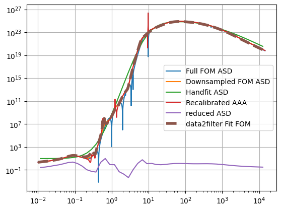
And plot the result

#_, TF_all = scipy.signal.freqs_zpk(all_z, all_p, k, worN = F_Hz)
#_, TF_minreal = scipy.signal.freqs_zpk(minreal_all_z, minreal_all_p, minreal_all_k, worN = F_Hz)


plt.loglog(F_bug, Div_PSD**0.5, label = "Full FOM ASD")
plt.loglog(F_FOM_dwn, FOM_ASD, label = "Downsampled FOM ASD")
plt.loglog(F_FOM_dwn, hand_xfr.mag, label = 'Handfit ASD')
plt.loglog(F_Hz, recalibrated_zpk_xfr.mag, label = 'Recalibrated AAA')
plt.loglog(F_FOM_dwn, reduced_ASD, label = "reduced ASD")
#plt.loglog(F_Hz, abs(TF_all), label = 'ALL ZPK Fit Bary. (order {})'.format(results.order))
#plt.loglog(F_Hz, abs(TF_minreal), label = 'Minreal ALL ZPK Fit Bary.', linestyle = '--')
plt.loglog(F_Hz, np.abs(iir_results.fitter.xfer_eval(F_Hz)), label = "data2filter Fit FOM", ls='--', linewidth=4)
plt.grid()
plt.legend()

<matplotlib.legend.Legend at 0x337d060b0>

iir_results.fitter.xfer_eval(F_Hz)

array([-8.40033252e-01-1.89162563e+00j,  8.80201515e-01-3.31859995e+00j,
        3.63020982e+00-3.82718193e+00j, ...,
       -6.28908229e+17-5.70991599e+19j, -6.28906692e+17-5.70990405e+19j,
       -6.28905155e+17-5.70989212e+19j], shape=(1450180,))

# Python code to merge dict using a single 
# expression
def Merge(dict1, dict2):
	res = {**dict1, **dict2}
	return res
	
# Driver code
dict1 = {'a': 10, 'b': 8}
dict2 = {'d': 6, 'c': 4}
dict3 = Merge(dict1, dict2)
print(dict3)
print(dict1)
print(dict2)

{'a': 10, 'b': 8, 'd': 6, 'c': 4}
{'a': 10, 'b': 8}
{'d': 6, 'c': 4}

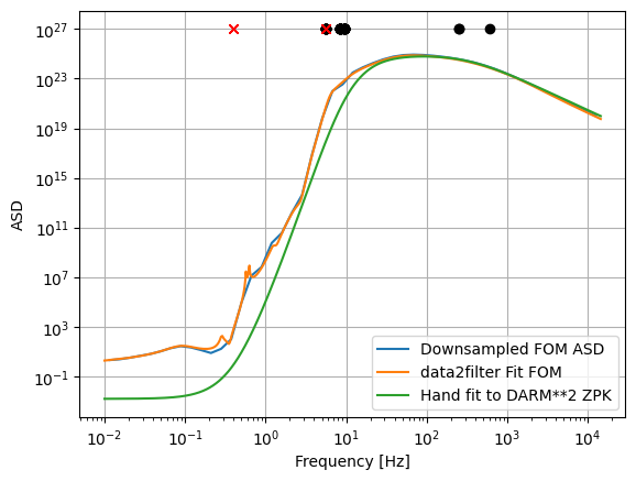
# Hand Fit the DARM**2 ZPK
shift_sq = 0.9
z_hand_sq = np.array([-0.07]*18) * 2 * np.pi * shift_sq
mp_sq = -0.75 -0.075j
mul_sq = 9
p_hand_sq = np.array([mp_sq]*mul_sq + [np.real(mp_sq)-np.imag(mp_sq)*1j]*mul_sq)*2 * 2 * np.pi * shift_sq
p_hand_sq = np.append(p_hand_sq, [-250]*2 +[-600]*1 + [-5000]*0)
# k_hand_sq = 9e39
k_hand_sq = 3e32

##making steeper roll off
mp_sq = mp_sq * 2.25
p_hand_sq = np.append(p_hand_sq, np.array([mp_sq]*8 +[np.real(mp_sq)-np.imag(mp_sq)*1j]*8+ [-1]*8)* 2 * np.pi * shift_sq)
z_hand_sq = np.append(z_hand_sq, np.array([-1]*24)* 2 * np.pi * shift_sq)

#k_hand_sq = k_hand_sq *1e9

#plt.loglog(F_bug, Div_PSD**0.5, label = "Full FOM ASD")
plt.loglog(F_FOM_dwn, FOM_ASD, label = "Downsampled FOM ASD")
#plt.loglog(F_Hz, abs(TF_all), label = 'ALL ZPK Fit Bary. (order {})'.format(results.order))
plt.loglog(F_Hz, np.abs(iir_results.fitter.xfer_eval(F_Hz)), label = "data2filter Fit FOM")
fq_plot = np.logspace(-2, 5, 10000)


hand_sys = SISO.zpk(z_hand_sq, p_hand_sq, k_hand_sq, convention='IIRrational')
#fr_hand = hand_sys.fresponse(f=fq_plot)
fr_hand = hand_sys.fresponse(f=F_bug)

plt.loglog(-np.real(p_hand_sq), np.array([1e27]*len(p_hand_sq)), color='black', linestyle='', marker='o')
plt.loglog(-np.real(z_hand_sq), np.array([1e27]*len(z_hand_sq)), color='r', linestyle='', marker='x')
plt.loglog(*fr_hand.fplot_mag, label = 'Hand fit to DARM**2 ZPK')
plt.xlabel("Frequency [Hz]")
plt.ylabel("ASD")

plt.grid()
plt.legend()

#plt.savefig('FOM_BNS_fit.pdf', bbox_inches='tight')

<matplotlib.legend.Legend at 0x3308a9360>

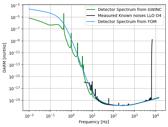
Next we calculate what this spectrum will look like from this FOM

LLO_O4_DARM = np.loadtxt('O4_data/L1_darm_measured.txt').T
LLO_O4_DARM_known = np.loadtxt('O4_data/L1_darm_known_measured.txt').T
LLO_O4_SUS_damping = np.loadtxt('O4_data/L1_sus_damping.txt').T

L_arm = 3995

det_PSD_from_FOM = (BNS_PSD/fr_hand.mag**2)**0.5
plt.loglog(F_bug, trace.psd**0.5*L_arm , label = 'Detector Spectrum from GWINC', color='green')
# plt.loglog(LLO_O4_DARM[0], LLO_O4_DARM[1]*L_arm , label = 'Measured DARM LLO O4', color='red')
# plt.loglog(LLO_O4_SUS_damping[0], LLO_O4_SUS_damping[1]*L_arm , label = 'SUS Damping', color='orange')
plt.loglog(LLO_O4_DARM_known[0], LLO_O4_DARM_known[1]*L_arm , label = 'Measured Known noises LLO O4', color='black')
plt.loglog(F_bug, det_PSD_from_FOM**0.5*L_arm , label = 'Detector Spectrum from FOM', color='dodgerblue')
plt.xlabel("Frequency [Hz]")
plt.ylabel("DARM [m/rtHz]")

# plt.xlim([6, 10000])
# plt.ylim([1e-20, 1e-15])


plt.grid()
plt.legend()

<matplotlib.legend.Legend at 0x337fc1690>

Now we will save our result so it can be loaded by the make full system example file

out_p = iir_results.fitter.poles.fullplane
out_z = iir_results.fitter.zeros.fullplane
out_k = iir_results.fitter.gain

# out_z = z_hand_sq
# out_p = p_hand_sq
# out_k = k_hand_sq

pre_save_sys = SISO.zpk(out_z, out_p, out_k, convention='IIRrational')
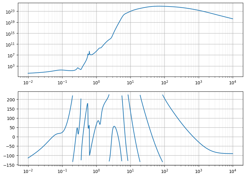
from wield.utilities.mpl import mplfigB
plotting_omega = np.logspace(-2, 4, 1000)
plt.close()
axB = mplfigB(Nrows = 2)
fr = pre_save_sys.fresponse(f=plotting_omega)
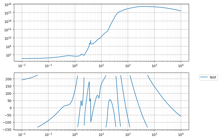
axB.ax0.loglog(*fr.fplot_mag, label='test')
axB.ax1.semilogx(*fr.fplot_deg225, label='test')


sys_save = SISO.zpk(out_z, out_p, out_k, convention='IIRrational')
zpk_dict = {
            'z' : [str(zero) for zero in np.asarray(tuple(sys_save.z)).tolist()],
            'p' : [str(pole) for pole in np.asarray(tuple(sys_save.p)).tolist()],
            'k' : float(sys_save.k)
            }

save('BNS_FOM.yml', zpk_dict)
#save('BNS_FOM_from_DARM.yml', zpk_dict)

Now it is saved. To open it use the following code

with open('BNS_FOM.yml', 'r') as file:
    filt_dict = yaml.safe_load(file)
p = np.array(filt_dict['p'], dtype=np.complex128)
z = np.array(filt_dict['z'], dtype=np.complex128)
k = np.float64(filt_dict['k'])
print(type(k))
print(len(z))
print(len(p))

print(k)
print(z)
print(p)

<class 'numpy.float64'>
49
52
-4.251712073985204e+34
[-1.71933238e+04+0.00000000e+00j -1.63099239e+04+0.00000000e+00j
 -1.29728162e+01+0.00000000e+00j -1.21499286e+01+0.00000000e+00j
 -7.55661313e-02+0.00000000e+00j -2.45521103e-02+0.00000000e+00j
 -2.48600198e+00+0.00000000e+00j -7.56379407e-02+0.00000000e+00j
 -2.48612066e+00+0.00000000e+00j -3.05765107e-01+6.60016416e-03j
 -3.05765107e-01-6.60016416e-03j -2.48486669e+00+9.73721622e-02j
 -2.48486669e+00-9.73721622e-02j -8.18777546e+01+8.99816240e+01j
 -8.18777546e+01-8.99816240e+01j -8.18777546e+01+8.99816240e+01j
 -8.18777546e+01-8.99816240e+01j -1.70409949e+00+1.71472024e+01j
 -1.70409949e+00-1.71472024e+01j -1.70409949e+00+1.71472024e+01j
 -1.70409949e+00-1.71472024e+01j -6.93961076e-02+2.22637834e+00j
 -6.93961076e-02-2.22637834e+00j -4.93047846e-01+1.67948889e+00j
 -4.93047846e-01-1.67948889e+00j -4.93047846e-01+1.67948889e+00j
 -4.93047846e-01-1.67948889e+00j -6.17306356e-01+8.52973777e+00j
 -6.17306356e-01-8.52973777e+00j -1.73319977e+01+5.90518075e+01j
 -1.73319977e+01-5.90518075e+01j -5.80500799e+02+3.59639192e+02j
 -5.80500799e+02-3.59639192e+02j -5.80500799e+02+3.59639192e+02j
 -5.80500799e+02-3.59639192e+02j -2.48486669e+00+9.73721622e-02j
 -2.48486669e+00-9.73721622e-02j -2.48486669e+00+9.73721622e-02j
 -2.48486669e+00-9.73721622e-02j -2.48486669e+00+9.73721622e-02j
 -2.48486669e+00-9.73721622e-02j -2.48486669e+00+9.73721622e-02j
 -2.48486669e+00-9.73721622e-02j -2.48486669e+00+9.73721622e-02j
 -2.48486669e+00-9.73721622e-02j -2.48486669e+00+9.73721622e-02j
 -2.48486669e+00-9.73721622e-02j -2.48486669e+00+9.73721622e-02j
 -2.48486669e+00-9.73721622e-02j]
[-1.26170405e-01  +0.j         -2.45290808e-02  +0.j
 -1.25665297e+04  +0.j         -1.26168860e-01  +0.j
 -8.03659898e+03+194.91460286j -8.03659898e+03-194.91460286j
 -2.37959049e+02  +6.39812641j -2.37959049e+02  -6.39812641j
 -9.60236922e+01  +2.28395724j -9.60236922e+01  -2.28395724j
 -1.25627968e+03 +33.14285309j -1.25627968e+03 -33.14285309j
 -5.32893506e+01  +5.46624111j -5.32893506e+01  -5.46624111j
 -6.49816520e+00 +38.83046579j -6.49816520e+00 -38.83046579j
 -6.49816520e+00 +38.83046579j -6.49816520e+00 -38.83046579j
 -3.00420896e-03  +3.93445773j -3.00420896e-03  -3.93445773j
 -1.63422797e-02  +3.57437107j -1.63422797e-02  -3.57437107j
 -2.46292757e-01  +0.50549057j -2.46292757e-01  -0.50549057j
 -2.46292757e-01  +0.50549057j -2.46292757e-01  -0.50549057j
 -5.61460029e-02  +1.7916299j  -5.61460029e-02  -1.7916299j
 -5.58553553e-01  +7.73696394j -5.58553553e-01  -7.73696394j
 -1.79345808e+01 +61.07755352j -1.79345808e+01 -61.07755352j
 -5.42617896e+02+121.0808547j  -5.42617896e+02-121.0808547j
 -5.42617896e+02+121.08085476j -5.42617896e+02-121.08085476j
 -5.32893506e+01  +5.46624111j -5.32893506e+01  -5.46624111j
 -5.32893506e+01  +5.46624111j -5.32893506e+01  -5.46624111j
 -5.32893506e+01  +5.46624111j -5.32893506e+01  -5.46624111j
 -5.32893506e+01  +5.46624111j -5.32893506e+01  -5.46624111j
 -5.32893506e+01  +5.46624111j -5.32893506e+01  -5.46624111j
 -5.32893506e+01  +5.46624111j -5.32893506e+01  -5.46624111j
 -5.32893506e+01  +5.46624111j -5.32893506e+01  -5.46624111j
 -5.32893506e+01  +5.46624111j -5.32893506e+01  -5.46624111j]

"""
This File has the sole purpose of creating the ASC DHARD Y Model that is then exported to the buzz repository.
"""

import os
import contextlib

import numpy as np
import matplotlib.pyplot as plt
import control

import pytest
import scipy
from scipy.signal import cheby2
from scipy import signal

from wield.bunch import Bunch
#from wield.control import MIMO
from wield.control import SISO
from wield.control.ss_bare.ss import BareStateSpace as RawStateSpace
from wield.control.ss_bare.ssprint import print_dense_nonzero
from wield.utilities.file_io import load, load_ls, save
from wield.utilities.mpl import mplfigB

from wield.pytest.fixtures import ( 
    tpath_join,
    plot,
    dprint,
    tpath,
    tpath_preclear,
    fpath_join,
    test_trigger,
)

from icecream import ic
from buzz import ssutil

import scipy.optimize
from wield.control import SISO


def bode(
    sys,
    axB=None,
    F_Hz=None,
    omega_limits=None,
    include_zp = True,
    label=None,
    **kwargs
):
    """
    sys should be a wield.control.SISO object
    """
    if axB is None:
        axB = mplfigB(Nrows = 2)

    if include_zp:
        z, p = sys._zp
        z = z[z.imag > 0]
        p = p[p.imag > 0]
        F_include = np.sort(np.concatenate(
            [
                z.imag,
                p.imag,
                z.imag - abs(z.real) - 1e-6,
                z.imag + abs(z.real) + 1e-6,
                p.imag - abs(p.real) - 1e-6,
                p.imag + abs(p.real) + 1e-6,
            ]
        )) / (2 * np.pi)
        F_include = F_include[F_include > 0]

        if omega_limits is None:
            omega_limits = (
                (F_include[0] + 1e-6) / 3,
                F_include[-1] * 3
            )

    if F_Hz is None:
        F_Hz = np.geomspace(omega_limits[0], omega_limits[1], 1000)

    if include_zp:
        print("F_include", F_include)
        F_Hz = np.sort(np.concatenate([F_Hz, F_include]))

    fr = sys.fresponse(f=F_Hz)
    axB.ax0.loglog(*fr.fplot_mag, label=label, **kwargs)
    if hasattr(axB, 'ax1'):
        axB.ax1.semilogx(*fr.fplot_deg225, label=label, **kwargs)
    return axB

FBNS_mod = SISO.zpk(z,p,k, convention='IIRrational')#.asSS
# FBNS_iod = {'F1.in':0, 'F1.out':0}
# FBNS = ssutil.makeSys(FBNS_mod, FBNS_iod)
# omega_lim = [min(F_Hz), max(F_Hz)]

#control.bode(FBNS.mod, Hz=True, wrap_phase=True, omega_limits=omega_lim)

from wield.utilities.mpl import mplfigB
plotting_omega = np.logspace(-2, 4, 1000)
plt.close()
axB = mplfigB(Nrows = 2)
fr = FBNS_mod.fresponse(f=plotting_omega)
axB.ax0.loglog(*fr.fplot_mag, label='test')
axB.ax1.semilogx(*fr.fplot_deg225, label='test')

# tol_list = range(10, 16)
# for tol in tol_list:
#     FBNS_tmp = ssutil.balance_sys_gain(FBNS, nr=tol)
#     nstates_tmp = FBNS.A.shape[0]
#     K_zpk_tmp = SISO.SISOStateSpace(BareStateSpace(FBNS_tmp.A, FBNS_tmp.B, FBNS_tmp.C, FBNS_tmp.D, None)).asZPK
#     control.bode(FBNS.mod, Hz=True, wrap_phase=True, omega_limits=omega_lim, label='sts: {}, tol: {}'.format(nstates_tmp, tol))

plt.legend(bbox_to_anchor=(1.05, 1), loc='upper left')
plt.savefig('postsave.png', dpi=300, bbox_inches='tight')
plt.show()
plt.close()