LIGO O4 Commissioning Paper
To make all plots from command line, run
jupyter execute plot.ipynb
import numpy as np
from numpy.random import randn, rand
import scipy as sp
import scipy.io as io
import scipy.signal

import matplotlib
import matplotlib.pyplot as plt
import matplotlib.gridspec as gridspec
from matplotlib.legend_handler import HandlerTuple
# import corner
# from wand.image import Image as WImage

import h5py


import os
import sys
from copy import deepcopy
# import time
# import csv
# import glob
import importlib
import warnings
warnings.filterwarnings("ignore")

# import emcee
# import multiprocessing
# import queue
# from itertools import count

import gwinc
#from gwinc.noise.quantum import shotrad_debug
import lib

## Set up plot
plt.rcdefaults()
matplotlib.rc('font',**{'family':'serif','serif':['Times'], 'size':16})
matplotlib.rc('text', usetex=True)
matplotlib.rc('lines', **{'ls':'-'})


L_arm = 3995

# h1nb = h5py.File("../data/noise_budget/lho_all_noisebudgets_gwinc_quantum.hdf5", 'r')
h1nb = h5py.File("data/noise_budget/lho_darm_noisebudget_O4a_hotOM2_start1386255618_span1800_median.hdf5", 'r')
l1nb = h5py.File("data/noise_budget/L1NB_G2400537.hdf5", 'r')

h1nb_xcorr = h5py.File("data/xcorr_budget/lho_correlated_darm_noisebudget_start1386718819_span900.hdf5", 'r')
xcorr = lib.DARM('data/xcorr_budget/1022_Unsqz.h5') # L1 xcorr


##############  Unify CTN  ##################
f_bin = np.geomspace(10, 1000, 100)

budget = gwinc.load_budget('Aplus')
aligo = gwinc.load_budget('aLIGO')
# CTN properly defined for O4 in "aLIGO" gwinc budget
budget.ifo.Materials = aligo.ifo.Materials

budget.freq = f_bin

# param, pcov = scipy.optimize.curve_fit(ctn, budget, mitctn, p0=[3.9e-4, 0.1])
# budget.ifo.Materials.Coating.Phihighn = param[0]
# budget.ifo.Materials.Coating.Phihighn_slope = param[1]

ctn_budget = deepcopy(budget)

# Unify AMD
def S_AMD(freq):
    return (2.32e-21*(100/freq)**0.5/L_arm)**2   # from wen
Noise budget
def h5_tree(val, pre=''):
    items = len(val)
    for key, val in val.items():
        items -= 1
        if items == 0:
            # the last item
            if type(val) == h5py._hl.group.Group:
                print(pre + '└── ' + key)
                h5_tree(val, pre+'    ')
            else:
                print(pre + '└── ' + key + ' (%d)' % len(val))
        else:
            if type(val) == h5py._hl.group.Group:
                print(pre + '├── ' + key)
                h5_tree(val, pre+'│   ')
            else:
                print(pre + '├── ' + key + ' (%d)' % len(val))


# filename = '../data/noise_budget/lho_all_noisebudgets_gwinc_quantum.hdf5'
# filename = '../data/noise_budget/L1NB_G2400537.hdf5'
filename = 'data/xcorr_budget/lho_correlated_darm_noisebudget_start1386718819_span900.hdf5'
with h5py.File(filename, 'r') as hf:
    print(hf)
    h5_tree(hf)

# hf = h5py.File(filename, 'r')
# for name in hf['H1/budget']:
#     print(name)
<HDF5 file "lho_correlated_darm_noisebudget_start1386718819_span900.hdf5" (mode r)>
├── CorrelatedDARM
│   ├── PSD (20000)
│   └── budget
│       ├── ASC
│       │   ├── PSD (20000)
│       │   └── budget
│       │       ├── CHARDPit
│       │       │   └── PSD (20000)
│       │       ├── CHARDYaw
│       │       │   └── PSD (20000)
│       │       ├── CSOFTPit
│       │       │   └── PSD (20000)
│       │       ├── CSOFTYaw
│       │       │   └── PSD (20000)
│       │       ├── DARMMeasured
│       │       │   └── PSD (20000)
│       │       ├── DHARDPit
│       │       │   └── PSD (20000)
│       │       ├── DHARDYaw
│       │       │   └── PSD (20000)
│       │       ├── DSOFTPit
│       │       │   └── PSD (20000)
│       │       ├── DSOFTYaw
│       │       │   └── PSD (20000)
│       │       ├── MICHPit
│       │       │   └── PSD (20000)
│       │       ├── MICHYaw
│       │       │   └── PSD (20000)
│       │       ├── PRC2Pit
│       │       │   └── PSD (20000)
│       │       ├── PRC2Yaw
│       │       │   └── PSD (20000)
│       │       ├── SRC2Pit
│       │       │   └── PSD (20000)
│       │       └── SRC2Yaw
│       │           └── PSD (20000)
│       ├── CalLines
│       │   ├── PSD (20000)
│       │   └── budget
│       │       ├── PCALX
│       │       │   └── PSD (20000)
│       │       └── PCALY
│       │           └── PSD (20000)
│       ├── CorrelatedDARMMeasured
│       │   └── PSD (20000)
│       ├── CorrelatedQuantum
│       │   └── PSD (20000)
│       ├── DARMMeasured
│       │   └── PSD (20000)
│       ├── DARMMeasuredO3bLHO_NoSQZ
│       │   └── PSD (20000)
│       ├── LSC
│       │   ├── PSD (20000)
│       │   └── budget
│       │       ├── DARMMeasured
│       │       │   └── PSD (20000)
│       │       ├── MICH
│       │       │   └── PSD (20000)
│       │       ├── PRCL
│       │       │   └── PSD (20000)
│       │       └── SRCL
│       │           └── PSD (20000)
│       ├── Laser
│       │   ├── PSD (20000)
│       │   └── budget
│       │       ├── DARMMeasured
│       │       │   └── PSD (20000)
│       │       ├── Frequency
│       │       │   └── PSD (20000)
│       │       ├── InputJitter
│       │       │   ├── PSD (20000)
│       │       │   └── budget
│       │       │       ├── DARMMeasured
│       │       │       │   └── PSD (20000)
│       │       │       ├── InputJitterPit
│       │       │       │   └── PSD (20000)
│       │       │       └── InputJitterYaw
│       │       │           └── PSD (20000)
│       │       └── Intensity
│       │           ├── PSD (20000)
│       │           └── budget
│       │               ├── DARMMeasured
│       │               │   └── PSD (20000)
│       │               ├── Intensity_high
│       │               │   └── PSD (20000)
│       │               ├── Intensity_low
│       │               │   └── PSD (20000)
│       │               └── Intensity_mid
│       │                   └── PSD (20000)
│       ├── OSEM
│       │   └── PSD (20000)
│       ├── PUMDAC
│       │   ├── PSD (20000)
│       │   └── budget
│       │       ├── ETMXPUMDAC
│       │       │   ├── PSD (20000)
│       │       │   └── budget
│       │       │       ├── DACModel18Bit
│       │       │       │   └── PSD (20000)
│       │       │       ├── ETMXLLPUMDAC
│       │       │       │   └── PSD (20000)
│       │       │       ├── ETMXLRPUMDAC
│       │       │       │   └── PSD (20000)
│       │       │       ├── ETMXULPUMDAC
│       │       │       │   └── PSD (20000)
│       │       │       ├── ETMXURPUMDAC
│       │       │       │   └── PSD (20000)
│       │       │       └── NoisemonADC
│       │       │           └── PSD (20000)
│       │       ├── ETMYPUMDAC
│       │       │   ├── PSD (20000)
│       │       │   └── budget
│       │       │       ├── DACModel18Bit
│       │       │       │   └── PSD (20000)
│       │       │       ├── ETMYLLPUMDAC
│       │       │       │   └── PSD (20000)
│       │       │       ├── ETMYLRPUMDAC
│       │       │       │   └── PSD (20000)
│       │       │       ├── ETMYULPUMDAC
│       │       │       │   └── PSD (20000)
│       │       │       ├── ETMYURPUMDAC
│       │       │       │   └── PSD (20000)
│       │       │       └── NoisemonADC
│       │       │           └── PSD (20000)
│       │       ├── ITMXPUMDAC
│       │       │   ├── PSD (20000)
│       │       │   └── budget
│       │       │       ├── DACModel18Bit
│       │       │       │   └── PSD (20000)
│       │       │       ├── ITMXLLPUMDAC
│       │       │       │   └── PSD (20000)
│       │       │       ├── ITMXLRPUMDAC
│       │       │       │   └── PSD (20000)
│       │       │       ├── ITMXULPUMDAC
│       │       │       │   └── PSD (20000)
│       │       │       ├── ITMXURPUMDAC
│       │       │       │   └── PSD (20000)
│       │       │       └── NoisemonADC
│       │       │           └── PSD (20000)
│       │       └── ITMYPUMDAC
│       │           ├── PSD (20000)
│       │           └── budget
│       │               ├── DACModel18Bit
│       │               │   └── PSD (20000)
│       │               ├── ITMYLLPUMDAC
│       │               │   └── PSD (20000)
│       │               ├── ITMYLRPUMDAC
│       │               │   └── PSD (20000)
│       │               ├── ITMYULPUMDAC
│       │               │   └── PSD (20000)
│       │               ├── ITMYURPUMDAC
│       │               │   └── PSD (20000)
│       │               └── NoisemonADC
│       │                   └── PSD (20000)
│       ├── ResidualGas
│       │   └── PSD (20000)
│       ├── Seismic
│       │   └── PSD (20000)
│       └── Thermal
│           ├── PSD (20000)
│           └── budget
│               ├── AMDBrownian
│               │   └── PSD (20000)
│               ├── CoatingBrownian
│               │   └── PSD (20000)
│               ├── CoatingThermoOptic
│               │   └── PSD (20000)
│               ├── DARMMeasured
│               │   └── PSD (20000)
│               ├── SubstrateBrownian
│               │   └── PSD (20000)
│               ├── SubstrateThermoElastic
│               │   └── PSD (20000)
│               └── SuspensionThermal
│                   ├── PSD (20000)
│                   └── budget
│                       ├── HorizPUM
│                       │   └── PSD (20000)
│                       ├── HorizTest mass
│                       │   └── PSD (20000)
│                       ├── HorizTop
│                       │   └── PSD (20000)
│                       ├── HorizUIM
│                       │   └── PSD (20000)
│                       ├── VertPUM
│                       │   └── PSD (20000)
│                       ├── VertTop
│                       │   └── PSD (20000)
│                       └── VertUIM
│                           └── PSD (20000)
└── Freq (20000)
dot = 0.8    # 1 is dense, 10 is sparsely distributed dots
lw1 = 2.0  # model curve
lw2 = 1.5  # measured curve
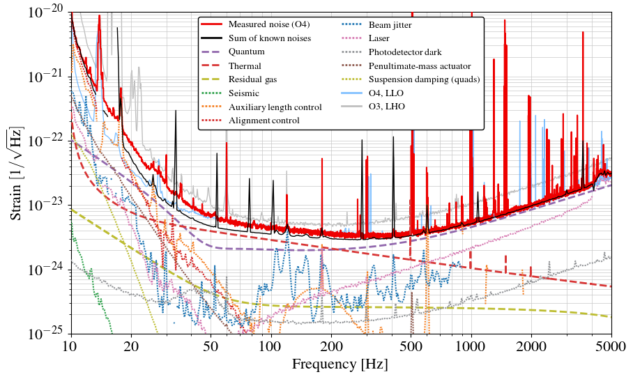
traces = {                              # color,                 linestyle, linewidth, zorder, lgdorder, label
    '/budget/DARMMeasured':             [[238/255,0/255,0/255]    ,         '-', 1.5,  10,  1, 'Measured noise (O4)'],
    '':                                 [[0/255,0/255,0/255]      ,         '-', 1.0, 100,  2, 'Sum of known noises'],
    '/budget/Quantum':                  [[146/255,104/255,173/255],        '--', lw1,  15,  3, 'Quantum'],
    '/budget/Thermal':                  [[216/255,54/255,54/255]  ,        '--', lw1,  16,  4, 'Thermal'],
    '/budget/ResidualGas':              [[189/255,189/255,50/255] ,        '--', lw1,  17,  5, 'Residual gas'],
    '/budget/Seismic':                  [[43/255,160/255,72/255]  , (0,(1,dot)), lw2,  30,  6, 'Seismic'],
    # '/budget/Newtonian':                [[33/255,191/255,207/255] ,         '-', 1.0, 5,  7, 'Newtonian'],
    '/budget/LSC':                      [[245/255,126/255,32/255] , (0,(1,dot)), lw2,  40,  8, 'Auxiliary length control'],
    '/budget/ASC':                      [[214/255,40/255,40/255]  , (0,(1,dot)), lw2,  50,  9, 'Alignment control'],
    '/budget/Laser/budget/InputJitter': [[32/255,119/255,180/255] , (0,(1,dot)), lw2,  50, 10, 'Beam jitter'],
    # '/budget/Laser/budget/Intensity':   [[43/255,160/255,72/255]  , (0,(1,dot)), lw2,   5, 12, 'Laser intensity'], # neg w/ freq noise
    '/budget/Laser/budget/Frequency':   [[214/255,121/255,177/255], (0,(1,dot)), lw2,  50, 13, 'Laser'],
    '/budget/Dark':                     [[147/255,149/255,152/255], (0,(1,dot)), lw2,  50, 14, 'Photodetector dark'],
    # '/budget/OMCLength':                [[0/255,0/255,0/255]      , (0,(1,dot)), lw2, 50, 15, 'Output mode cleaner length'],
    '/budget/PUMDAC':                   [[141/255,88/255,77/255]  , (0,(1,dot)), lw2,  50, 16, 'Penultimate-mass actuator'],
    '/budget/OSEM':                     [[189/255,189/255,50/255] , (0,(1,dot)), lw2,  50, 17, 'Suspension damping (quads)'],
}


S_calLines = h1nb_xcorr['CorrelatedDARM']['budget']['CalLines']['PSD'][:]/L_arm**2

freq = np.geomspace(10,5000,500)
trace = ctn_budget.run(freq=freq)
S_thermal = S_AMD(freq) + trace.CoatingBrownian.psd + trace.SuspensionThermal.psd + trace.CoatingThermoOptic.psd + trace.SubstrateBrownian.psd + trace.SubstrateThermoElastic.psd


for key in traces:
    psd = lib.DARM()
    psd.f = h1nb['Freq'][:]
    psd.S = h1nb['H1'+key+'/PSD'][:]/L_arm**2

    fmt = traces[key]

    if 'ASC' in key:
        psd.S[(psd.f >= 13.5) & (psd.f <= 18)] = np.nan

    if key=='': # for the black sum of known noises trace
        psd.S -= S_calLines
        psd.S[(psd.f >= 13.4) & (psd.f <= 14.5)] = np.nan
        psd.S[(psd.f >= 15.2) & (psd.f <= 17.1)] = np.nan
        psd.S[(psd.f >= 33) & (psd.f <= 34) & (psd.S<1e-45)] = np.nan
        psd.S -= h1nb['H1/budget/Thermal/PSD'][:]/L_arm**2
        psd.setZeroErr(); psd.rebin_log2log(freq)
        psd.S += S_thermal

    if key == 'Thermal':
        plt.loglog(freq, np.sqrt(S_thermal), c=fmt[0], ls=fmt[1], lw=fmt[2], zorder=fmt[3], label=fmt[5], alpha=1)
        continue


    lgdorder = fmt[4]

    if lgdorder > 5:
        psd.setZeroErr(); psd.rebin_log2log(freq)

    plt.loglog(psd.f, np.sqrt(psd.S), c=fmt[0], ls=fmt[1], lw=fmt[2], zorder=fmt[3], label=fmt[5], alpha=1)


plt.loglog(l1nb['Freq'][:], np.sqrt(l1nb['L1/budget/DARMMeasured/PSD'][:]/L_arm**2),
           c=[75/255,166/255,255/255], alpha=0.7, lw=1.0, zorder=3, label='O4, LLO')

np.savetxt('L1_darm_measured.txt', np.array([l1nb['Freq'][:], np.sqrt(l1nb['L1/budget/DARMMeasured/PSD'][:]/L_arm**2)]).T)
np.savetxt('L1_darm_known_measured.txt', np.array([l1nb['Freq'][:], np.sqrt(l1nb['L1//PSD'][:]/L_arm**2)]).T)
np.savetxt('L1_sus_damping.txt', np.array([l1nb['Freq'][:], np.sqrt(l1nb['L1/budget/OSEM/PSD'][:]/L_arm**2)]).T)


# plot LHO O3a strain
h1o3 = np.loadtxt("data/noise_budget/2019-09-05_H1_O3a_darm_displacement_paperData.txt")
plt.plot(h1o3[:,0][::5] , h1o3[:,1][::5]/L_arm, alpha=0.5, c='grey', lw=1, zorder=0, label='O3, LHO')#[75/255,166/255,255/255],


plt.xlabel('Frequency [Hz]')
plt.ylabel(r'Strain $\mathrm{[1/\sqrt{Hz}]}$')
# plt.title('(a) LIGO Hanford Observatory (LHO)', fontsize=16)

plt.xticks([10,20,50,100,200,500,1000,2000,5000], ('10','20','50','100','200','500','1000','2000','5000'))
plt.xlim(10, 5000)
plt.ylim(1e-25, 1e-20)

grayrgb = 200
plt.grid(True, which='both', color=[grayrgb/255,grayrgb/255,grayrgb/255], linestyle='-', linewidth=0.5)


legend = plt.legend(loc='upper center', fontsize=10, edgecolor='black', ncol=2, handlelength=2, markerscale=3)
for line in legend.get_lines(): line.set_linewidth(2)
legend.bbox_to_anchor=(0.5, 1.25)
legend.set_zorder(1000)
legend.get_frame().set_alpha(None)
legend.get_frame().set_facecolor('white')


plt.gcf().set_size_inches(10, 6)

plt.savefig('H1_noise_budget.svg', bbox_inches='tight')
plt.savefig('H1_noise_budget.pdf', bbox_inches='tight')
plt.show()
import lib, importlib; importlib.reload(lib)

dot = 0.8   # 1 is dense, 10 is sparsely distributed dots
lw1 = 2.0  # model curve
lw2 = 1.5  # measured curve
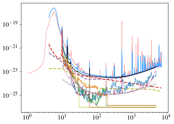
traces = {         # color,                    linestyle, linewidth, zorder, lgdorder, label
    '/budget/DARMMeasured':             [[75/255,166/255,255/255] ,         '-', 1.5,  10,  1, 'Measured noise (O4)'],
    '':                                 [[0/255,0/255,0/255]      ,         '-', 1.0, 100,  2, 'Sum of known noises'],
    '/budget/Quantum':                  [[146/255,104/255,173/255],        '--', lw1,  15,  3, 'Quantum'],
    '/budget/Thermal':                  [[216/255,54/255,54/255]  ,        '--', lw1,  16,  4, 'Thermal'],
    '/budget/ResidualGas':              [[189/255,189/255,50/255] ,        '--', lw1,  17,  5, 'Residual gas'],
    '/budget/Seismic':                  [[43/255,160/255,72/255]  , (0,(1,dot)), lw2,  14,  6, 'Seismic'],
    # '/budget/Newtonian':                [[33/255,191/255,207/255] ,         '-', 1.0, 5,  7, 'Newtonian'],
    '/budget/LSC':                      [[245/255,126/255,32/255] , (0,(1,dot)), lw2,  50,  8, 'Auxiliary length control'],
    '/budget/ASC':                      [[214/255,40/255,40/255]  , (0,(1,dot)), lw2,  50,  9, 'Alignment control'],
    '/budget/Laser/budget/InputJitter': [[32/255,119/255,180/255] , (0,(1,dot)), lw2,  50, 10, 'Beam jitter'],
    # '/budget/Laser/budget/Intensity':   [[43/255,160/255,72/255]  , (0,(1,dot)), lw2,  50, 12, 'Laser intensity'],
    '/budget/Laser':                    [[214/255,121/255,177/255], (0,(1,dot)), lw2,  50, 13, 'Laser'], # freq + RIN
    '/budget/Dark':                     [[147/255,149/255,152/255], (0,(1,dot)), lw2,  50, 14, 'Photodetector dark'],
    # '/budget/FCBackscatter':            [[90/255,70/255,90/255]   , (0,(1,dot)), lw2,  50, 15, 'Filter cavity backscatter'],
    '/budget/PUMDAC':                   [[141/255,88/255,77/255]  , (0,(1,dot)), lw2,  50, 16, 'Penultimate-mass actuator'],
    '/budget/OSEM':                     [[189/255,189/255,50/255] , (0,(1,dot)), lw2,  50, 17, 'Suspension damping (quads+triples)'],
}


freq = np.geomspace(10,5000,500)
trace = ctn_budget.run(freq=freq)
S_thermal = S_AMD(freq) + trace.CoatingBrownian.psd + trace.SuspensionThermal.psd + trace.CoatingThermoOptic.psd + trace.SubstrateBrownian.psd + trace.SubstrateThermoElastic.psd


for key in traces:
    psd = lib.DARM()
    psd.f = l1nb['Freq'][:]
    psd.S = l1nb['L1'+key+'/PSD'][:]/L_arm**2

    fmt = traces[key]

    if key=='': # for the black sum of known noises trace
        psd.S -= l1nb['L1/budget/Thermal/PSD'][:]/L_arm**2
        psd.setZeroErr(); psd.rebin_log2log(freq)
        psd.S += S_thermal

    if key == 'Thermal':
        plt.loglog(freq, np.sqrt(S_thermal), c=fmt[0], ls=fmt[1], lw=fmt[2], zorder=fmt[3], label=fmt[5], alpha=1)
        continue

    lgdorder = fmt[4]
    if lgdorder > 5:
        psd.setZeroErr(); psd.rebin_log2log(freq)

    plt.loglog(psd.f, np.sqrt(psd.S), c=fmt[0], ls=fmt[1], lw=fmt[2], zorder=fmt[3], label=fmt[5], alpha=1)


plt.loglog(h1nb['Freq'][:], np.sqrt(h1nb['H1/budget/DARMMeasured/PSD'][:]/L_arm**2),
           c=[238/255,0/255,0/255], alpha=0.4, lw=1.0, zorder=3, label='O4, LHO')


# plot LLO O3a strain, copied from O3 commish paper
NB_LLO_O3 = io.loadmat('../data/noise_budget/LLO_O3_NB_data.mat',squeeze_me=True, struct_as_record=False)
freqq     = NB_LLO_O3['NB'].freq
darm_o3_0 = NB_LLO_O3['NB'].DARM_reference/L_arm
darm_o3   = np.interp(freq, freqq, darm_o3_0)
plt.loglog(freq, darm_o3, alpha=0.5, lw=1, c='grey', zorder=0, label='O3, LLO')


plt.xlabel('Frequency [Hz]')
plt.ylabel(r'Strain $\mathrm{[1/\sqrt{Hz}]}$')
# plt.title('(b) LIGO Livingston Observatory (LLO)', fontsize=16)

plt.xticks([10,20,50,100,200,500,1000,2000,5000], ('10','20','50','100','200','500','1000','2000','5000'))
plt.xlim(10, 5000)
plt.ylim(1e-25, 1e-20)

grayrgb = 200
plt.grid(True, which='both', color=[grayrgb/255,grayrgb/255,grayrgb/255], linestyle='-', linewidth=0.5)


# legend = plt.legend([handles[idx] for idx in order],[labels[idx] for idx in order], fontsize=13*fontscale, edgecolor='black', ncol=3)
legend = plt.legend(loc='upper center', fontsize=10, edgecolor='black', ncol=2, handlelength=2, markerscale=3)
for line in legend.get_lines(): line.set_linewidth(2)
legend.bbox_to_anchor=(0.5, 1.25)
# legend = ax.legend(edgecolor="black", fontsize=10)
legend.set_zorder(1000)
legend.get_frame().set_alpha(None)
legend.get_frame().set_facecolor('white')


plt.gcf().set_size_inches(10, 6)


plt.savefig('L1_noise_budget.svg', bbox_inches='tight')
plt.savefig('L1_noise_budget.pdf', bbox_inches='tight')
plt.show()
---------------------------------------------------------------------------
FileNotFoundError                         Traceback (most recent call last)
File ~/miniconda3/envs/controls/lib/python3.10/site-packages/scipy/io/matlab/_mio.py:39, in _open_file(file_like, appendmat, mode)
     38 try:
---> 39     return open(file_like, mode), True
     40 except OSError as e:
     41     # Probably "not found"

FileNotFoundError: [Errno 2] No such file or directory: '../data/noise_budget/LLO_O3_NB_data.mat'

During handling of the above exception, another exception occurred:

FileNotFoundError                         Traceback (most recent call last)
Cell In[4], line 62
     56 plt.loglog(h1nb['Freq'][:], np.sqrt(h1nb['H1/budget/DARMMeasured/PSD'][:]/L_arm**2),
     57            c=[238/255,0/255,0/255], alpha=0.4, lw=1.0, zorder=3, label='O4, LHO')
     61 # plot LLO O3a strain, copied from O3 commish paper
---> 62 NB_LLO_O3 = io.loadmat('../data/noise_budget/LLO_O3_NB_data.mat',squeeze_me=True, struct_as_record=False)
     63 freqq     = NB_LLO_O3['NB'].freq
     64 darm_o3_0 = NB_LLO_O3['NB'].DARM_reference/L_arm

File ~/miniconda3/envs/controls/lib/python3.10/site-packages/scipy/io/matlab/_mio.py:225, in loadmat(file_name, mdict, appendmat, **kwargs)
     88 """
     89 Load MATLAB file.
     90
   (...)
    222     3.14159265+3.14159265j])
    223 """
    224 variable_names = kwargs.pop('variable_names', None)
--> 225 with _open_file_context(file_name, appendmat) as f:
    226     MR, _ = mat_reader_factory(f, **kwargs)
    227     matfile_dict = MR.get_variables(variable_names)

File ~/miniconda3/envs/controls/lib/python3.10/contextlib.py:135, in _GeneratorContextManager.__enter__(self)
    133 del self.args, self.kwds, self.func
    134 try:
--> 135     return next(self.gen)
    136 except StopIteration:
    137     raise RuntimeError("generator didn't yield") from None

File ~/miniconda3/envs/controls/lib/python3.10/site-packages/scipy/io/matlab/_mio.py:17, in _open_file_context(file_like, appendmat, mode)
     15 @contextmanager
     16 def _open_file_context(file_like, appendmat, mode='rb'):
---> 17     f, opened = _open_file(file_like, appendmat, mode)
     18     try:
     19         yield f

File ~/miniconda3/envs/controls/lib/python3.10/site-packages/scipy/io/matlab/_mio.py:45, in _open_file(file_like, appendmat, mode)
     43     if appendmat and not file_like.endswith('.mat'):
     44         file_like += '.mat'
---> 45     return open(file_like, mode), True
     46 else:
     47     raise OSError(
     48         'Reader needs file name or open file-like object'
     49     ) from e

FileNotFoundError: [Errno 2] No such file or directory: '../data/noise_budget/LLO_O3_NB_data.mat'
traces = {         # color,                    linestyle, linewidth, zorder, lgdorder, label
    '':                                 [[0/255,0/255,0/255]      ,        '-', 1.0, 5,  2, 'Sum of known noises'],
    '/budget/ASC':                      [[214/255,40/255,40/255]  , (0,(1,10)), 1.0, 5,  9, 'Alignment control'],
    '/budget/DARMMeasured':             [[32/255,119/255,180/255] ,        '-', 1.0, 5,  1, 'Measured noise (O4)'],
    '/budget/Dark':                     [[147/255,149/255,152/255], (0,(1,10)), 1.0, 5, 14, 'Photodetector dark'],
    '/budget/LSC':                      [[245/255,126/255,32/255] , (0,(1,10)), 1.0, 5, 8 , 'Auxiliary length control'],
    '/budget/Laser/budget/Frequency':   [[214/255,121/255,177/255], (0,(1,10)), 1.0, 5, 13, 'Laser frequency'],
    '/budget/Laser/budget/InputJitter': [[32/255,119/255,180/255] , (0,(1,10)), 1.0, 5, 10, 'Beam jitter'],
    '/budget/OMCLength':                [[0/255,0/255,0/255]      , (0,(1,10)), 1.0, 5, 15, 'Output mode cleaner length'],
    '/budget/PUMDAC':                   [[141/255,88/255,77/255]  , (0,(1,10)), 1.0, 5, 16, 'Penultimate-mass actuator'],
    '/budget/Quantum':                  [[146/255,104/255,173/255],        '-', 1.0, 5,  3, 'Quantum'],
    '/budget/ResidualGas':              [[189/255,189/255,50/255] ,        '-', 1.0, 5,  7, 'Residual gas'],
    '/budget/Seismic':                  [[43/255,160/255,72/255]  ,        '-', 1.0, 5,  5, 'Seismic'],
    '/budget/Thermal':                  [[216/255,54/255,54/255]  ,        '-', 1.0, 5,  4, 'Thermal'],
    # '/budget/Newtonian':                [[33/255,191/255,207/255] ,        '-', 1.0, 5,  5, 'Newtonian'],
}


freq = h1nb['Freq'][:]

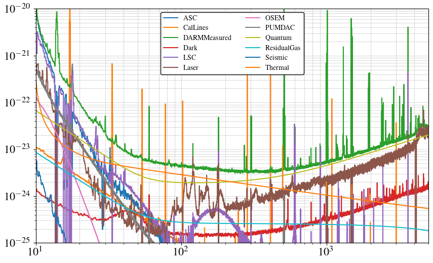
for name, data in h1nb['H1/budget'].items():
    plt.loglog(freq, np.sqrt(data['PSD'][:])/L_arm, label=name)

# for key in traces:
#     fmt = traces[key]
#     plt.loglog(freq, np.sqrt(data['H1'+key+'/PSD'][:])/L_arm, c=fmt[0], ls=fmt[1], lw=fmt[2], zorder=fmt[3], label=fmt[4])

plt.xlim(10, 5000)
plt.ylim(1e-25, 1e-20)

grayrgb = 200
plt.grid(True, which='both', color=[grayrgb/255,grayrgb/255,grayrgb/255], linestyle='-', linewidth=0.5)


# legend = plt.legend([handles[idx] for idx in order],[labels[idx] for idx in order], fontsize=13*fontscale, edgecolor='black', ncol=3)
legend = plt.legend(fontsize=10, edgecolor='black', ncol=2)
# legend.loc='upper center'
legend.bbox_to_anchor=(0.5, 1.25)
# legend = ax.legend(edgecolor="black", fontsize=10)
# legend.set_zorder(100)
legend.get_frame().set_alpha(None)
legend.get_frame().set_facecolor('white')


plt.gcf().set_size_inches(10, 6)


# plt.savefig('test.svg')
# plt.savefig('test.pdf')
plt.show()
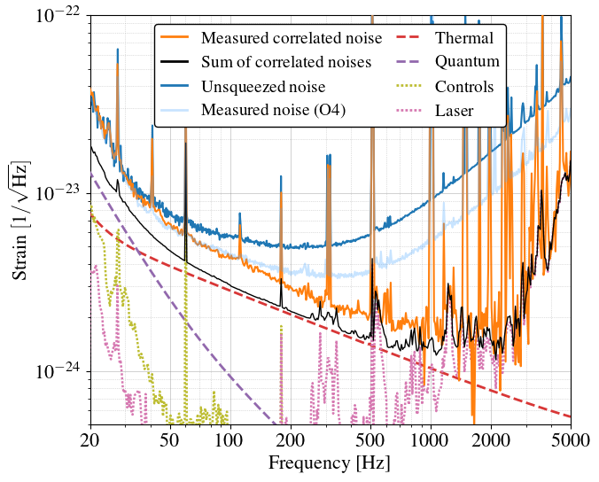
Correlated noise budget
Compute xcorr from raw time series, and correct it by making sum and GDS-STRAIN equal
f_bin = np.geomspace(10, 5000, 500)


dot = 0.8  # 1 is dense, 10 is sparsely distributed dots
lw1 = 2.0  # model curve
lw2 = 1.8  # measured curve

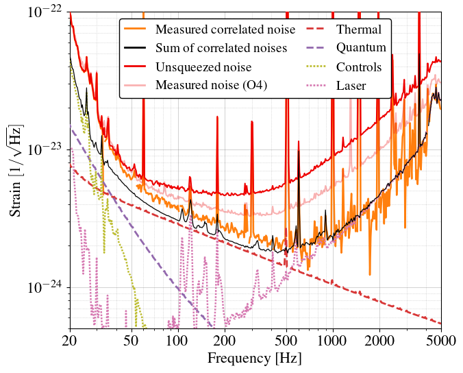
traces = {                        # color,                    linestyle, linewidth, zorder, lgdorder, label
    '/budget/CorrelatedDARMMeasured':   ['#ff7f0e',                           '-', lw2, 5, 1, 'Measured correlated noise'],
    # '/budget/DARMMeasuredO3bLHO_NoSQZ': ['grey',                              '-', 1,   5, 1, 'O3, Unsqueezed noise'],
    '/budget/DARMMeasured':             [[238/255,0/255,0/255] ,              '-', 1.5, 100, 0, 'Unsqueezed noise'],
    # '':                                 [[0/255,0/255,0/255] ,              '-',   1.0, 5,  2, 'Sum of known noises'],
    '/budget/CorrelatedQuantum':        [[146/255,104/255,173/255],          '--', lw1, 5,  3, 'Quantum'],
    '/budget/Thermal':                  [[216/255,54/255,54/255]  ,          '--', lw1, 5,  4, 'Thermal'],
    '/budget/ResidualGas':              [[189/255,189/255,50/255] ,          '--', lw1, 0,  5, 'Residual gas'],
    '/budget/Seismic':                  [[43/255,160/255,72/255],     (0,(1,dot)), lw2, 5,  6, 'Seismic'],
    '/budget/Newtonian':                [[33/255,191/255,207/255],          '-', 1.0, 5,  7, 'Newtonian'],
    '/budget/LSC':                      [[245/255,126/255,32/255] ,   (0,(1,dot)), lw2, 5,  8, 'Auxiliary length control'],
    '/budget/ASC':                      [[214/255,40/255,40/255],     (0,(1,dot)), lw2, 5,  9, 'Alignment control'],
    '/budget/Laser/budget/InputJitter': [[32/255,119/255,180/255] ,   (0,(1,dot)), lw2, 5, 10, 'Beam jitter'],
    '/budget/Laser/budget/Intensity':   [[43/255,160/255,72/255],     (0,(1,dot)), lw2, 5, 12, 'Laser intensity'],
    '/budget/Laser/budget/Frequency':   [[214/255,121/255,177/255],   (0,(1,dot)), lw2, 6, 13, 'Laser frequency'],
    '/budget/PUMDAC':                   [[141/255,88/255,77/255],     (0,(1,dot)), lw2, 5, 16, 'Penultimate-mass actuator'],
    '/budget/OSEM':                     [[189/255,189/255,50/255],    (0,(1,dot)), lw2, 5, 17, 'Suspension damping (quads)'],
}


trace = ctn_budget.run(freq=f_bin)
S_thermal = S_AMD(f_bin) + trace.CoatingBrownian.psd + trace.SuspensionThermal.psd + trace.CoatingThermoOptic.psd + trace.SubstrateBrownian.psd + trace.SubstrateThermoElastic.psd


# Subtract CTN and CAL lines from "sum of expected noises"
S_thermal_h1 = h1nb_xcorr['CorrelatedDARM']['budget']['Thermal']['PSD'][:]
S_calLines   = h1nb_xcorr['CorrelatedDARM']['budget']['CalLines']['PSD'][:]

psd = lib.DARM()
psd.f = h1nb_xcorr['Freq'][:]
psd.S = h1nb_xcorr['CorrelatedDARM']['PSD'][:]  # black line, sum of known noises
psd.S -= S_thermal_h1
psd.S -= S_calLines
psd.setZeroErr(); psd.rebin_log2log(f_bin)

psd.S += S_thermal*L_arm**2
S_sum = deepcopy(psd.S)

# S_sum = 0
# for key in traces:
#     fmt = traces[key]
#     lgdorder = fmt[4]
#     if lgdorder > 2:
#         S_sum += h1nb_xcorr['CorrelatedDARM'+key+'/PSD'][:]
#         # S_sum += h1nb['H1'+key+'/PSD'][:]/L_arm**2

# combine laser and controls noises
laser_keys=['/budget/Laser/budget/InputJitter',
            '/budget/Laser/budget/Intensity',
            '/budget/Laser/budget/Frequency']
S_laser = 0
for key in laser_keys:
    S_laser += h1nb_xcorr['CorrelatedDARM'+key+'/PSD'][:]/L_arm**2
psd = lib.DARM()
psd.f = h1nb_xcorr['Freq'][:]; psd.S = S_laser
psd.setZeroErr(); psd.rebin_log2log(f_bin)
S_laser = psd.S

controls_keys=['/budget/LSC',
               '/budget/ASC',
               '/budget/PUMDAC',
               '/budget/OSEM']
S_controls = 0
for key in controls_keys:
    S_controls += h1nb_xcorr['CorrelatedDARM'+key+'/PSD'][:]/L_arm**2
psd = lib.DARM()
psd.f = h1nb_xcorr['Freq'][:]; psd.S = S_controls
psd.setZeroErr(); psd.rebin_log2log(f_bin)
S_controls = psd.S


plot_keys=['/budget/CorrelatedDARMMeasured',
           '/budget/DARMMeasured',
           '/budget/Thermal',
           '/budget/CorrelatedQuantum',
           '/budget/OSEM',
        #    '/budget/Laser/budget/InputJitter',
           '/budget/Laser/budget/Frequency',]


for key in plot_keys:
    psd = lib.DARM()
    psd.f = h1nb_xcorr['Freq'][:]
    psd.S = h1nb_xcorr['CorrelatedDARM'+key+'/PSD'][:]/L_arm**2

    if key == '/budget/CorrelatedDARMMeasured':   # remove cal lines from meas corr noise
        psd.S[(psd.f >= 78.5) & (psd.f <= 79)] = np.nan
        psd.S -= S_calLines/L_arm**2


    fmt = traces[key]
    lgdorder = fmt[4]
    if lgdorder >= 0:  # rebin traces
        psd.setZeroErr(); psd.rebin_log2log(f_bin)

    if key == '/budget/Laser/budget/Frequency':
        plt.loglog(f_bin, np.sqrt(S_laser), c=fmt[0], ls=fmt[1], lw=fmt[2], zorder=fmt[3], label='Laser')
        continue

    if key == '/budget/OSEM':
        plt.loglog(f_bin, np.sqrt(S_controls), c=fmt[0], ls=fmt[1], lw=fmt[2], zorder=fmt[3], label='Controls')
        continue


    # if key == '/budget/DARMMeasured' or 'O3' in key: alpha=0.3   # fade unsqz noise
    plt.loglog(psd.f, np.sqrt(psd.S), c=fmt[0], ls=fmt[1], lw=fmt[2], zorder=fmt[3], label=fmt[5], alpha=1)


    if key == '/budget/CorrelatedDARMMeasured':  # orange
        psd.S[(psd.f >= 78.5) & (psd.f <= 79)] = np.nan
        S_sum[(psd.f >= 4090) & (psd.f <= 4100)] = np.nan
        plt.loglog(f_bin, np.sqrt(S_sum/L_arm**2), c='black', ls='-', lw=0.9, zorder=200, label='Sum of correlated noises')

        # # plot LHO O3a strain
        # h1o3 = np.loadtxt("../data/noise_budget/2019-09-05_H1_O3a_darm_displacement_paperData.txt")
        # plt.plot(h1o3[:,0][::6] , h1o3[:,1][::6]/L_arm, alpha=0.35, c='grey', lw=1, zorder=0, label='O3, Squeezed noise')


    elif key == '/budget/DARMMeasured':   # if plotting unsqz, then plot sqz total noise after
        psd_h1 = lib.DARM()
        psd_h1.f = h1nb['Freq'][:]
        psd_h1.S = np.sqrt(h1nb['H1/budget/DARMMeasured/PSD'][:]/L_arm**2)
        psd_h1.setZeroErr(); psd_h1.rebin_log2log(f_bin)

        plt.loglog(psd_h1.f, psd_h1.S,
           c=[238/255,0/255,0/255], ls=fmt[1], lw=fmt[2], zorder=fmt[3], label='Measured noise (O4)', alpha=0.3)


plt.xlabel('Frequency [Hz]')
plt.ylabel(r'Strain $\mathrm{[1/\sqrt{Hz}]}$')
# # plt.title('(a) LIGO Hanford Observatory', fontsize=16)

# plt.xticks([10,20,50,100,200,500,1000,2000,5000], ('10','20','50','100','200','500','1000','2000','5000'))
# plt.xlim(20, 5000)

# plt.yticks([1e-26, 1e-25, 1e-24, 1e-23, 1e-22, 1e-21, 1e-20,])
# ax=plt.gca()
# ax.yaxis.set_minor_locator(matplotlib.ticker.LogLocator(numticks=999, subs="auto"))
# plt.ylim(1e-25, 1e-21)

plt.xticks([10,20,50,100,200,500,1000,2000,5000], ('10','20','50','100','200','500','1000','2000','5000'))
plt.xlim(20, 5000)
plt.ylim(5e-25, 1e-22)

plt.grid(which='major', color='grey', alpha=0.5, ls='-', lw=0.5)
plt.grid(which='minor', color='grey', alpha=0.5, ls=':', lw=0.5)

legend = plt.legend(loc='upper center', fontsize=14, edgecolor='black',
                    ncol=2, handlelength=1.5, markerscale=3, columnspacing=0.8,)
for line in legend.get_lines(): line.set_linewidth(2)
legend.bbox_to_anchor=(0.5, 1.25)
legend.set_zorder(1000)
legend.get_frame().set_alpha(None)
legend.get_frame().set_facecolor('white')


# plt.gcf().set_size_inches(10, 6)
plt.gcf().set_size_inches(7, 6)

plt.savefig('H1_xcorr_budget.svg', bbox_inches='tight')
plt.savefig('H1_xcorr_budget.pdf', bbox_inches='tight')
plt.show()
import lib, importlib; importlib.reload(lib)


folder = '../data/xcorr_budget/';
filelist = [
        # # '0514_0_FDS',
        # '0514_1_Unsqz_FCmis_LOonCLF',
        # # '0514_2_FIS',
        # # '0514_3_FIAS',
        # # '0514_4_FIS_minus140',
        # '0514_5_Unsqz_FCmis_LOonCLF',
        # # '0514_6_FIS_minus150',
        # # '0514_7_FIS_minus170',
        # # '0514_8_FIS_minus140',
        # '0514_9_Unsqz_FCmis_LOonCLF',
        # # '0514_10_QND_minus30',
        # # '0514_11_QND_minus50',
        # # '0514_12_QND_plus100',
        # '0514_13_Unsqz_FCmis_LOonCLF',
        # # '0514_14_QND_plus143',
        # # '0514_15_QND_plus140',
        # # '0514_16_QND_plus140', # Lost lock after this
        # '0514_17_Unsqz_FCmis_LOonCLF',
        # # '0514_18_QND_plus200',
        # # '0514_19_QND_plus250',
        # '0514_20_Unsqz_FCmis_LOonCLF',
        # # '0514_21_FDS',
        # # '0514_22_FDS',
        # '0514_23_Unsqz_FCmis_LOonCLF',
        # # '0514_24_QND_plus40',
        # '0514_25_Unsqz_FCmis_LOonCLF',
        # # '0514_26_QND_plus70',
        # '0514_27_Unsqz_FCmis_LOonCLF',
        # # '0514_28_QND_plus140',
        # '0514_29_Unsqz_FCmis_LOonCLF',
        # # '0514_30_QND_plus170', # Lost lock
        # # '0515_1_FDS',
        # # '0515_2_Unsqz_FConRLF_LOengaged',
        # # '0515_3_FDS',
        # '0515_4_Unsqz_FConRLF_LOengaged',
        # '0515_5_Unsqz_FCmis_LOfinalized', # Lost lock
        # '0516_1_Unsqz_FCmis_LOfinalized',
        # '0516_2_Unsqz_FCmis_LOfinalized',
        # '0516_3_Unsqz_FCmis_LOfinalized',
        # '0516_4_Unsqz_FCmis_LOfinalized',
        # '0516_5_Unsqz_FCmis_LOfinalized',
        # '0516_6_Unsqz_FCmis_LOfinalized',
        # '0516_7_Unsqz_FCmis_LOfinalized',
        # '0516_8_Unsqz_FCmis_LOfinalized',
        # '0516_9_Unsqz_FCmis_LOfinalized',
        # '0516_10_Unsqz_FCmis_LOfinalized', # Lost lock
        # # '0522_1_Unsqz_FConRLFCLF',
        # '0522_2_Unsqz_FConRLFCLF_CLF5.0_gain4_FCBST_LO0dB',
        # '0522_3_Unsqz_FConRLFCLF_CLF3.94_gain4_FCBST_LO0dB',
        # '0522_4_Unsqz_FCmis_CLF3.94_gain6_LO2dB',
        # '0522_5_Unsqz_FCmis_CLF3.94_gain1_LOm10dB', # Lost lock
        # '0523_1_FDS',
        # '0523_2_FIS',
        # '0523_3_FIAS',
        # '0523_4_FDAS',
        # '0523_5_FDS_angle1',
        # '0523_6_FDS_angle2',
        # '0523_7_FDS_angle3',
        # '0523_8_Unsqz_FConRLFCLF_LOengaged',
        # '0523_9_Unsqz_FConRLFCLF_LOengaged_PRX',
        '1022_Unsqz'
    ]
fileext = '.mat'


# filelist = ['0516_1_Unsqz_FCmis_LOfinalized']


# calCorrect = np.loadtxt('./data/calibration/L1_uncertainty_systematic_correction.txt')
# freq = calCorrect[:,0]
# real = calCorrect[:,1]
# imag = calCorrect[:,2]

# mag = abs(real + 1j*imag)
# mag[0] = np.nan
# mag[-1] = np.nan # No extrapolation
# phi = np.angle(real + 1j*imag)*180/np.pi


# darkNoise = np.loadtxt('./data/dark/dark_20230411.txt', delimiter=',')
# ff = darkNoise[:,0]
# S_dark = darkNoise[:,1]**2
# S_dark[0] = np.nan
# S_dark[-1] = np.nan

for name in filelist:
    if not os.path.isfile(folder + name + '.h5'):

        darm = lib.DARM(folder + name + fileext)
        darm.welch(deltaf=2**(-4))

    #     darm.calCorrect = np.interp(darm.f, freq, mag)
    #     calfile = glob.glob('./data/calibration/' + name + '*.txt')
    #     caldata = np.loadtxt(calfile[0]) # f, median mag, median phi, 16th mag, 16th phi, 84th mag, 84th phi
    #     darm.calMedian = np.interp(darm.f, caldata[:,0], caldata[:,1])

        # darm.S = darm.S*darm.calCorrect**2*darm.calMedian**2 # mag is ASD strain correction. We square here because it's systematic error instead of random error
    #     darm.relerrG_n = abs(np.interp(darm.f, caldata[:,0], caldata[:,3])*darm.calCorrect-1)*2 # x2 because PSD relative error. Not square cuz it's random error
    #     darm.relerrG_p = (np.interp(darm.f, caldata[:,0], caldata[:,5])*darm.calCorrect-1)*2

        darm.welch_sum(average='median')
        # darm.S_sum = abs(darm.S_sum*darm.calCorrect**2*darm.calMedian**2)

        GDSoverCAL = darm.S/darm.S_sum # Compensate sys err on PD
        # GDSoverCAL = 1

        darm.S_sum = darm.S_sum*GDSoverCAL

        darm.welch_null(average='median')
        darm.S_null = darm.S_null*GDSoverCAL
        # darm.S_null = darm.S_null*darm.calCorrect**2*darm.calMedian**2

        darm.xcorr(average='mean')
        darm.S_xcorr = np.real(darm.S_xcorr)*GDSoverCAL
        # darm.S_xcorr = np.real(darm.S_xcorr)*darm.calCorrect**2*darm.calMedian**2

        # darm.S_dark = np.interp(darm.f, ff, S_dark)*darm.calCorrect**2*darm.calMedian**2

        # darm.S_shot = darm.S - darm.S_xcorr - darm.S_dark
        # darm.S_shot = darm.S_null - darm.S_dark

        darm.save(folder + name + '.h5')
f_bin = np.geomspace(10, 5000, 500)

xcorr = lib.DARM('../data/xcorr_budget/1022_Unsqz.h5')
unsqz = deepcopy(xcorr)
# unsqz.removeLines('DARM'); unsqz.removeLines('CAL');
unsqz.rebin_log(np.geomspace(10, 5000, 750))

xcorr.S = xcorr.S_xcorr
# xcorr.removeLines('DARM'); xcorr.removeLines('CAL');
xcorr.rebin_log(f_bin)


budget = gwinc.load_budget("../data/noise_budget/L1_1022_FC7000.yaml")
budget.ifo.Squeezer.Type='None'
traces = budget.run()
sr = shotrad_debug(f_bin, budget.ifo)
ASbudget = sr.ASbudget
loss = (
    ASbudget.lossSEC + ASbudget.lossARM + ASbudget.Loss_injection
    + ASbudget.Loss_readout + ASbudget.lossMM
)
qnoise = sr.Gamma_IFO * sr.etaS_full + loss
S_xqn = (sr.PSDdisplacement * (qnoise - 1))/(L_arm)**2
S_xqn = np.real(S_xqn)
S_xqn[S_xqn < 0] = 0

dot = 0.8  # 1 is dense, 10 is sparsely distributed dots
lw1 = 2.0  # model curve
lw2 = 1.8  # measured curve
traces = {                               # color,                    linestyle, linewidth, zorder, lgdorder, label
    '/budget/DARMMeasured':             [[75/255,166/255,255/255] ,         '-', 1.5, 100,  1, 'Measured noise (O4)'],
    # '':                                 [[0/255,0/255,0/255]      ,         '-', 1.0, 5,  2, 'Sum of known noises'],
    '/budget/Quantum':                  [[146/255,104/255,173/255],        '--', lw1, 5,  3, 'Quantum'],
    '/budget/Thermal':                  [[216/255,54/255,54/255]  ,        '--', lw1,   5,  4, 'Thermal'],
    '/budget/ResidualGas':              [[189/255,189/255,50/255] ,        '--', lw1,   2,  5, 'Residual gas'],
    '/budget/Seismic':                  [[43/255,160/255,72/255]  , (0,(1,dot)), lw2, 5,  6, 'Seismic'],
    # '/budget/Newtonian':                [[33/255,191/255,207/255] ,         '-', 1.0, 5,  7, 'Newtonian'],
    '/budget/LSC':                      [[245/255,126/255,32/255] , (0,(1,dot)), lw2,   5,  8, 'Auxiliary length control'],
    '/budget/ASC':                      [[214/255,40/255,40/255]  , (0,(1,dot)), lw2,   5,  9, 'Alignment control'],
    '/budget/Laser/budget/InputJitter': [[32/255,119/255,180/255] , (0,(1,dot)), lw2,   5, 10, 'Beam jitter'],
    '/budget/Laser/budget/Intensity':   [[43/255,160/255,72/255]  , (0,(1,dot)), lw2,   5, 12, 'Laser intensity'],
    '/budget/Laser':                    [[214/255,121/255,177/255], (0,(1,dot)), lw2,   5, 13, 'Laser frequency'], # Freq + RIN
    # '/budget/Dark':                     [[147/255,149/255,152/255], (0,(1,dot)), lw2, 5, 14, 'Photodetector dark'],
    # '/budget/FCBackscatter':                [[0/255,0/255,0/255]  , (0,(1,dot)), lw2, 1, 15, 'Filter cavity backscatter'],
    '/budget/PUMDAC':                   [[141/255,88/255,77/255]  , (0,(1,dot)), lw2, 5, 16, 'Penultimate-mass actuator'],
    '/budget/OSEM':                      [[189/255,189/255,50/255] , (0,(1,dot)), lw2, 5, 17, 'Suspension damping (quads+triples)'],
}

# file = io.loadmat('../data/thermal/l1nbws_nov23.mat');
# temp = file['ff']
# freq = np.reshape(temp, temp.size)
# temp = file['thermal_amd_to_darm']
# S_amd = np.interp(f_bin, freq, np.reshape(temp, temp.size))**2
# temp = file['thermal_sus_to_darm']
# S_sus = np.interp(f_bin, freq, np.reshape(temp, temp.size))**2
# S_ctn_fit = (1.75e-20*(100/f_bin)**0.54/L_arm)**2
# S_thermal_fit = S_ctn_fit + S_amd + S_sus

# NB = h5py.File('../data/noise_budget/gwincNBdata.h5', 'r')
# sub_freq = NB['SubBrown']['Freq'][:]
# sub      = NB['SubBrown']['PSD'][:]
# S_sub = np.interp(f_bin, sub_freq, sub)**2
# # ctn_freq = NB['CoatBrown']['Freq'][:]
# # ctn = np.sqrt(NB['CoatBrown']['PSD'][:])/L_arm
# S_thermal_fit = S_ctn_fit + S_amd + S_sus + S_sub


plt.loglog(xcorr.f, np.sqrt(abs(xcorr.S)), ls='-', c='#ff7f0e', lw=1.5, zorder=10, label='Measured correlated noise')

# combine laser and controls noises
laser_keys=['/budget/Laser/budget/InputJitter',
            '/budget/Laser/budget/Intensity',
            '/budget/Laser']
S_laser = 0
for key in laser_keys:
    S_laser += l1nb['L1'+key+'/PSD'][:]/L_arm**2
psd = lib.DARM()
psd.f = l1nb['Freq'][:]; psd.S = S_laser
psd.setZeroErr(); psd.rebin_log2log(f_bin)
S_laser = psd.S

controls_keys=['/budget/LSC',
               '/budget/ASC',
               '/budget/PUMDAC',
               '/budget/OSEM']
S_controls = 0
for key in controls_keys:
    S_controls += l1nb['L1'+key+'/PSD'][:]/L_arm**2
psd = lib.DARM()
psd.f = l1nb['Freq'][:]; psd.S = S_controls
psd.setZeroErr(); psd.rebin_log2log(f_bin)
S_controls = psd.S


trace = ctn_budget.run(freq=f_bin)
S_thermal = S_AMD(f_bin) + trace.CoatingBrownian.psd + trace.SuspensionThermal.psd + trace.CoatingThermoOptic.psd + trace.SubstrateBrownian.psd + trace.SubstrateThermoElastic.psd


S_sum = 0
for key in traces:
    fmt = traces[key]
    lgdorder = fmt[4]
    if lgdorder >= 4:
        S_sum += l1nb['L1'+key+'/PSD'][:]/L_arm**2


# Use fit instead
psd = lib.DARM()
psd.f = l1nb['Freq'][:]; psd.S = S_sum
psd.S -= l1nb['L1/budget/Thermal/PSD'][:]/L_arm**2
psd.setZeroErr(); psd.rebin_log2log(f_bin)
psd.S = psd.S + S_thermal + abs(S_xqn)


plt.loglog(psd.f, np.sqrt(psd.S), c='black', ls='-', lw=1.0, zorder=20, label='Sum of correlated noises')

plt.loglog(unsqz.f, np.sqrt(unsqz.S), ls='-', alpha=1.0, lw=1.5, zorder=2, label='Unsqueezed noise')


plot_keys=['/budget/DARMMeasured',
           '/budget/Thermal',
           '/budget/Quantum',
           '/budget/OSEM',
        #    '/budget/Laser/budget/InputJitter',
        #    '/budget/Laser/budget/Intensity',
           '/budget/Laser']

# for key in traces:
for key in plot_keys:
    psd = lib.DARM()
    psd.f = l1nb['Freq'][:]
    psd.S = l1nb['L1'+key+'/PSD'][:]/L_arm**2

    fmt = traces[key]

    lgdorder = fmt[4]
    if lgdorder == 1 or lgdorder>5:
        psd.setZeroErr(); psd.rebin_log2log(f_bin)

    if key == '/budget/DARMMeasured':
        plt.loglog(psd.f, np.sqrt(psd.S), c=fmt[0], ls=fmt[1], lw=fmt[2], zorder=fmt[3], label=fmt[5], alpha=0.3)
        continue

    if key == '/budget/Thermal':
        plt.loglog(f_bin, np.sqrt(S_thermal), c=fmt[0], ls=fmt[1], lw=fmt[2], zorder=fmt[3], label='Thermal')
        # plt.loglog(f_bin, np.sqrt(S_thermal_fit), c=fmt[0], ls='dotted', lw=fmt[2], zorder=fmt[3], label='Thermal (fit)')

        continue

    if key == '/budget/Laser':
        plt.loglog(f_bin, np.sqrt(S_laser), c=fmt[0], ls=fmt[1], lw=fmt[2], zorder=fmt[3], label='Laser')
        continue

    if key == '/budget/OSEM':
        plt.loglog(f_bin, np.sqrt(S_controls), c=fmt[0], ls=fmt[1], lw=fmt[2], zorder=fmt[3], label='Controls')
        continue

    if key == '/budget/Quantum':
        plt.loglog(f_bin, np.sqrt(S_xqn), c=[146/255,104/255,173/255], ls='--', lw=2.0, zorder=5, label=fmt[5])
        continue

    plt.loglog(psd.f, np.sqrt(psd.S), c=fmt[0], ls=fmt[1], lw=fmt[2], zorder=fmt[3], label=fmt[5])


plt.xlabel('Frequency [Hz]')
plt.ylabel(r'Strain $\mathrm{[1/\sqrt{Hz}]}$')
# plt.title('(b) LIGO Livingston Observatory', fontsize=16)

plt.xticks([10,20,50,100,200,500,1000,2000,5000], ('10','20','50','100','200','500','1000','2000','5000'))
plt.xlim(20, 5000)
plt.ylim(5e-25, 1e-22)

plt.grid(which='major', color='grey', alpha=0.5, ls='-', lw=0.5)
plt.grid(which='minor', color='grey', alpha=0.5, ls=':', lw=0.5)

legend = plt.legend(loc='upper center', fontsize=14, edgecolor='black',
                    ncol=2, handlelength=1.5, markerscale=3, columnspacing=0.8,)
for line in legend.get_lines(): line.set_linewidth(2)
legend.bbox_to_anchor=(0.5, 1.25)
legend.set_zorder(1000)
legend.get_frame().set_alpha(None)
legend.get_frame().set_facecolor('white')


# plt.gcf().set_size_inches(10, 6)
plt.gcf().set_size_inches(7, 6)


plt.savefig('L1_xcorr_budget.svg', bbox_inches='tight')
plt.savefig('L1_xcorr_budget.pdf', bbox_inches='tight')
plt.show()
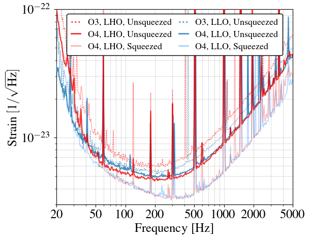
## Compare O3 vs. O4 without and with squeezing
flo_compare_sndarm = 850
fhi_compare_sndarm = 950
print(f"comparing shot-noise-limited strains between {flo_compare_sndarm} - {fhi_compare_sndarm} Hz\n")


f_bin = np.geomspace(15, 5000, 400)

plt.rcdefaults()
matplotlib.rc('font',**{'family':'serif','serif':['Times'], 'size':18})
matplotlib.rc('text', usetex=True)


dot = 1.5

# unsqueezed O3  LHO
o3lho_unsqz = lib.DARM()
o3lho_unsqz.f = h1nb_xcorr['Freq'][:]
o3lho_unsqz.S = h1nb_xcorr['CorrelatedDARM']['budget']['DARMMeasuredO3bLHO_NoSQZ']['PSD'][:]/L_arm**2
o3lho_unsqz.setZeroErr(); o3lho_unsqz.rebin_log2log(f_bin)
plt.loglog(o3lho_unsqz.f, o3lho_unsqz.S**0.5, c='red', alpha=0.8, ls=(0,(1,dot)), lw=1., zorder=20, label='O3, LHO, Unsqueezed')
o3lho_nosqz_asd = np.nanmedian(o3lho_unsqz.S[(o3lho_unsqz.f >= flo_compare_sndarm) & (o3lho_unsqz.f <= fhi_compare_sndarm)])**0.5
print(f"{o3lho_nosqz_asd*1e23=:0.5f}")

# unsqueezed O4  LHO
o4lho_unsqz = lib.DARM()
o4lho_unsqz.f = h1nb_xcorr['Freq'][:]
o4lho_unsqz.S = h1nb_xcorr['CorrelatedDARM']['budget']['DARMMeasured']['PSD'][:]/L_arm**2
o4lho_unsqz.setZeroErr(); o4lho_unsqz.rebin_log2log(f_bin)
plt.loglog(o4lho_unsqz.f, o4lho_unsqz.S**0.5, c=[238/255,0/255,0/255], alpha=0.8, lw=1.5, zorder=200, label='O4, LHO, Unsqueezed')
o4lho_nosqz_asd = np.nanmedian(o4lho_unsqz.S[(o4lho_unsqz.f >= flo_compare_sndarm) & (o4lho_unsqz.f <= fhi_compare_sndarm)])**0.5
print(f"{o4lho_nosqz_asd*1e23=:0.5f}")

# squeezed O4  LHO
o4lho = lib.DARM()
o4lho.f = h1nb['Freq'][:]
o4lho.S = h1nb['H1/budget/DARMMeasured/PSD'][:]/L_arm**2
o4lho.setZeroErr(); o4lho.rebin_log2log(f_bin)
plt.loglog(o4lho.f, o4lho.S**0.5, zorder=1, alpha=0.3, c=[238/255,0/255,0/255], lw=1, label='O4, LHO, Squeezed') #[238/255,0/255,0/255])


# unsqueezed O3  LLO, from O3 commish paper
# O3 Cross correlation measured + noise budget from 2019-03-24
NB_LLO_O3nosqz = io.loadmat('../data/noise_budget/LLO_O3_NB_data_nosqz.mat',squeeze_me=True,struct_as_record=False)
o3llo_nosqz = lib.DARM()
o3llo_nosqz.f = NB_LLO_O3nosqz['NB'].freq
o3llo_nosqz.S =(NB_LLO_O3nosqz['NB'].DARM_reference/L_arm)**2
o3llo_nosqz.setZeroErr(); o3llo_nosqz.rebin_log2log(f_bin)
plt.loglog(o3llo_nosqz.f, o3llo_nosqz.S**0.5, c='C0', alpha=0.8, ls=(0,(1,dot)), lw=1., zorder=10, label='O3, LLO, Unsqueezed')
o3llo_nosqz_asd = np.nanmedian(o3llo_nosqz.S[(o3llo_nosqz.f >= flo_compare_sndarm) & (o3llo_nosqz.f <= fhi_compare_sndarm)])**0.5
print(f"{o3llo_nosqz_asd*1e23=:0.5f}")

# unsqueezed O4  LLO
xcorr = lib.DARM('../data/xcorr_budget/1022_Unsqz.h5')
unsqz = deepcopy(xcorr)
unsqz.rebin_log(f_bin)
plt.loglog(unsqz.f, np.sqrt(unsqz.S), c='C0', lw=1.5, alpha=0.8, zorder=190, label='O4, LLO, Unsqueezed')
o4llo_nosqz_asd = np.nanmedian(unsqz.S[(unsqz.f >= flo_compare_sndarm) & (unsqz.f <= fhi_compare_sndarm)])**0.5
print(f"{o4llo_nosqz_asd*1e23=:0.5f}")

# squeezed O4  LLO
o4llo = lib.DARM()
o4llo.f = l1nb['Freq'][:]
o4llo.S = l1nb['L1/budget/DARMMeasured/PSD'][:]/L_arm**2
o4llo.setZeroErr(); o4llo.rebin_log2log(f_bin)
plt.loglog(o4llo.f, o4llo.S**0.5, alpha=0.5, zorder=0, c=[75/255,166/255,255/255], lw=1, label='O4, LLO, Squeezed') #, c=[75/255,166/255,255/255]


plt.xlabel('Frequency [Hz]')
plt.ylabel(r'Strain $\mathrm{[1/\sqrt{Hz}]}$')

plt.xticks([10,20,50,100,200,500,1000,2000,5000], ('10','20','50','100','200','500','1000','2000','5000'))
plt.xlim(20, 5000)
plt.ylim(3e-24, 1e-22)
# plt.yticks([1e-24, 1e-23, 1e-22,])
# ax=plt.gca()
# ax.yaxis.set_minor_locator(matplotlib.ticker.LogLocator(numticks=999, subs="auto"))
# plt.ylim(1e-25, 1e-21)


plt.grid(True, which='both', color='grey', linestyle=':', linewidth=0.5)
# plt.grid(which='major', color='grey', alpha=0.7, ls='-', lw=0.5)
# plt.grid(which='minor', color='grey', alpha=0.5, ls=':', lw=0.5)

legend = plt.legend(loc='upper center', fontsize=13, edgecolor='black', ncol=2, handlelength=1.,
                    columnspacing=.8, labelspacing=0.4, borderpad=0.5)
for line in legend.get_lines(): line.set_linewidth(2)
legend.bbox_to_anchor=(0.5, 1.25)
legend.set_zorder(1000)
legend.get_frame().set_alpha(None)
legend.get_frame().set_facecolor('white')


plt.gcf().set_size_inches(6, 5)

plt.savefig('compare_sqz_unsqz.svg', bbox_inches='tight')
plt.savefig('compare_sqz_unsqz.pdf', bbox_inches='tight')

print()
print(f"{(o3llo_nosqz_asd/o4llo_nosqz_asd)**2=:0.5f}")
print(f"{(o3lho_nosqz_asd/o4lho_nosqz_asd)**2=:0.5f}")

print()
print(f"{220*(o3llo_nosqz_asd/o4llo_nosqz_asd)**2=:0.5f}")
print(f"{190*(o3lho_nosqz_asd/o4lho_nosqz_asd)**2=:0.5f}")
comparing shot-noise-limited strains between 850 - 950 Hz

o3lho_nosqz_asd*1e23=1.13707
o4lho_nosqz_asd*1e23=0.82150
o3llo_nosqz_asd*1e23=0.97124
o4llo_nosqz_asd*1e23=0.83841

(o3llo_nosqz_asd/o4llo_nosqz_asd)**2=1.34195
(o3lho_nosqz_asd/o4lho_nosqz_asd)**2=1.91582

220*(o3llo_nosqz_asd/o4llo_nosqz_asd)**2=295.22951
190*(o3lho_nosqz_asd/o4lho_nosqz_asd)**2=364.00573
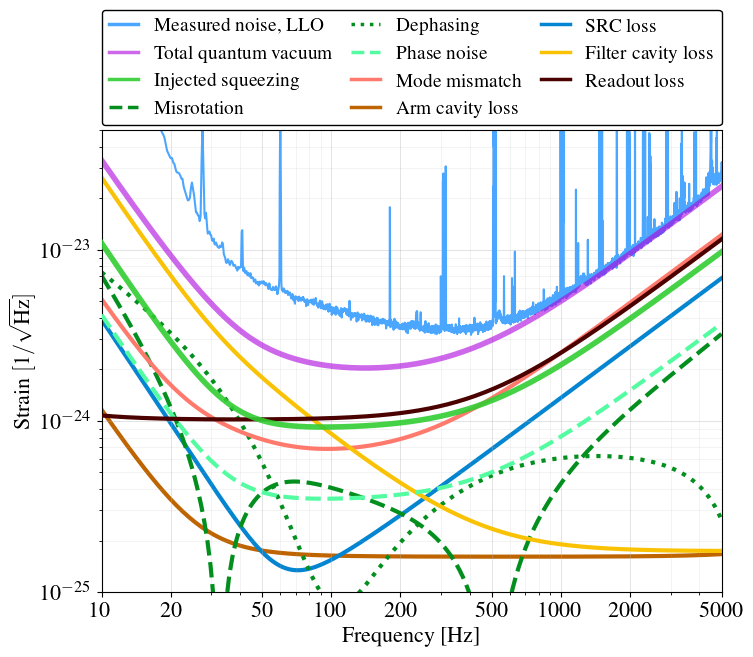
Quantum noise budget
# savedata = False

## Set up plot
matplotlib.rc('font',**{'family':'serif','serif':['Times'], 'size':16})
matplotlib.rc('text', usetex=True)
matplotlib.rc('lines', **{'ls':'-'})

# budget = gwinc.load_budget('L1_0514_FC7000.yaml')
budget = gwinc.load_budget("../data/noise_budget/L1_1022_FC7000.yaml")
freq = np.geomspace(10, 5000, 200)
# sqz_ang_deg = lib.getAngleSqzHighFreq(budget)
# print(sqz_ang_deg, sqz_ang_deg/180*np.pi)
# budget.ifo.Squeezer.SQZAngle = 15*np.pi/180
# print(budget.ifo.Squeezer.FilterCavity.L_mm)
# budget.ifo.Squeezer.FilterCavity.fdetune = -45
# budget.ifo.Squeezer.FilterCavity.loss = -45
trace = budget.run(freq=freq)


fig = plt.figure()
psd = lib.DARM()
psd.f = l1nb['Freq'][:]
psd.S = l1nb['L1/budget/DARMMeasured/PSD'][:]/L_arm**2
plt.loglog(psd.f, np.sqrt(psd.S), lw=1.5, c=[75/255,166/255,255/255], label='Measured noise, LLO')

ax = fig.gca()
fig = trace.Quantum.plot(ax);
handles, previous_labels = ax.get_legend_handles_labels()
print(f"{previous_labels = }")


ax.lines[2].set_color('limegreen')  # inj squeezing
ax.lines.pop(-2) #  Injection loss (cut)
ax.lines.pop(6)  #  SQZ FC Length RMS*
ax.lines.pop(6)  #  SQZ SEC Length RMS*, given the above SQZ FC Length RMS* has been removed
ax.lines[-3].set_zorder(0) # fc loss
# ax.lines[-4].set_color('xkcd:cerulean') # sec loss
ax.lines[-5].set_color('xkcd:salmon')  # mode mismatch
ax.lines[-4].set_zorder(0)     # arm loss
ax.lines[2].set_linewidth(4)   # gen sqz
ax.lines[2].set_alpha(0.9)     # gen sqz
ax.lines[2].set_linewidth(4)   # gen sqz
ax.lines[2].set_zorder(20)     # gen sqz
ax.lines[-1].set_zorder(19)    # readout loss
ax.lines[5].set_zorder(15)     # phase noise
# ax.lines[5].set_color('lawngreen') # phase noise

fig.set_size_inches(8, 6)


handles, previous_labels = ax.get_legend_handles_labels()
new_labels = previous_labels
new_labels = [  'Measured noise, LLO',
                'Total quantum vacuum',
                'Injected squeezing', #'Generated SQZ',
                'Misrotation', #'Anti-SQZ*', #'SQZ misrotation*',
                'Dephasing', #'SQZ FC/IFO dephasing*',
                'Phase noise',
                'Mode mismatch',
                'Arm cavity loss',
                'SRC loss',
                'Filter cavity loss',
                # 'Injection loss',
                'Readout loss']
legend = plt.legend(handles=handles, labels=new_labels, loc=[0, 1.01],#'lower center',
                    fontsize=14, ncol=3, columnspacing=1, handlelength=1.5, edgecolor='black',)
# legend = plt.legend(loc='lower center', fontsize=12, ncol=3, handlelength=1.5, edgecolor='black',)
for line in legend.get_lines(): line.set_linewidth(2.5)
legend.set_zorder(1000)
legend.get_frame().set_alpha(None)
legend.get_frame().set_facecolor('white')
print(f"{new_labels = }")

plt.ylabel(r'Strain $\mathrm{[1/\sqrt{Hz}]}$')
plt.ylim(1e-25, 5e-23)
plt.xticks([10,20,50,100,200,500,1000,2000,5000], ('10','20','50','100','200','500','1000','2000','5000'));


plt.savefig('./L1_qn_subbudget.svg', bbox_inches='tight')
plt.savefig('./L1_qn_subbudget.pdf', bbox_inches='tight')
print(f'modelled sqz angle @ {budget.ifo.Squeezer.SQZAngle*180/np.pi:0.5f} deg')
previous_labels = ['Measured noise, LLO', 'Total Quantum Vacuum', 'AS Port SQZ', 'SQZ misrotation*', 'SQZ FC/IFO dephasing*', 'SQZ Phase Noise*', 'SQZ FC Length RMS*', 'SQZ SEC Length RMS*', 'Mode Mismatch', 'Arm Loss', 'SEC Loss', 'Filter Cavity Loss', 'Injection Loss', 'Readout Loss']
new_labels = ['Measured noise, LLO', 'Total quantum vacuum', 'Injected squeezing', 'Misrotation', 'Dephasing', 'Phase noise', 'Mode mismatch', 'Arm cavity loss', 'SRC loss', 'Filter cavity loss', 'Readout loss']
modelled sqz angle @ -11.00000 deg
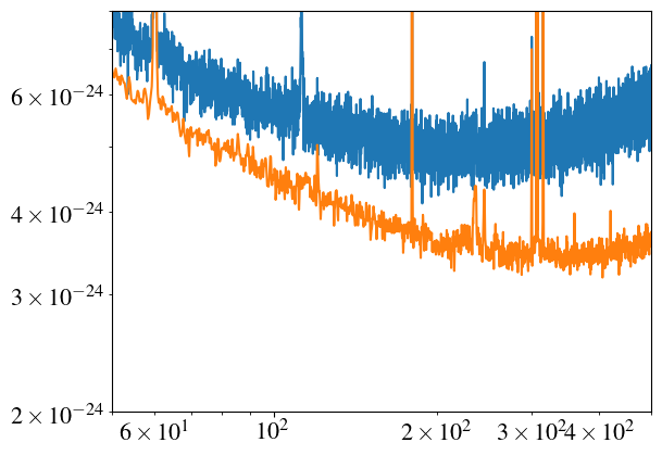
Thermal noise & Fitting mid-freq noise
plt.loglog(xcorr.f, abs(np.sqrt(xcorr.S)))

# psd = lib.DARM()
# psd.f = h1nb_xcorr['Freq'][:]
# key = '/budget/CorrelatedDARMMeasured'
# psd.S = h1nb_xcorr['CorrelatedDARM'+key+'/PSD'][:]/L_arm**2

plt.loglog(psd.f, abs(np.sqrt(psd.S)))

plt.xlim(50,500)
plt.ylim(2e-24, 8e-24)
plt.show()
def ctn(f, A,e):
    return A*(100/f)**e


# L1 xcorr
f_bin = np.geomspace(60, 300, 60)

xcorr = lib.DARM('../data/xcorr_budget/1022_Unsqz.h5')
# unsqz = deepcopy(xcorr)
# unsqz.removeLines('DARM'); unsqz.removeLines('CAL');
xcorr.S = xcorr.S_xcorr
xcorr.removeLines('DARM');
xcorr.rebin_log(f_bin)

# re-calculate correlated quantum noise
# can then subtract it from xcorr, and fit remaining excess
budget = gwinc.load_budget("../data/noise_budget/L1_1022_FC7000.yaml")
budget.ifo.Squeezer.Type='None'
traces = budget.run(f=f_bin)
sr = shotrad_debug(f_bin, budget.ifo)
ASbudget = sr.ASbudget
loss = (
    ASbudget.lossSEC + ASbudget.lossARM + ASbudget.Loss_injection
    + ASbudget.Loss_readout + ASbudget.lossMM
)
qnoise = sr.Gamma_IFO * sr.etaS_full + loss
S_xqn = (sr.PSDdisplacement * (qnoise - 1))/(L_arm)**2
S_xqn = np.real(S_xqn)
S_xqn[S_xqn < 0] = 0

# xcorr.S -= S_xqn

l1ctn, pcov = scipy.optimize.curve_fit(ctn, xcorr.f, L_arm*np.sqrt(abs(xcorr.S)), p0=[1.1e-20, 0.45])


plt.loglog(f_bin, L_arm*np.sqrt(abs(xcorr.S)), c=[75/255,166/255,255/255], lw=1.5, zorder=10, label='Measured correlated noise, LLO')
plt.loglog(f_bin, ctn(f_bin, *l1ctn), c=[75/255,166/255,255/255], ls='--', lw=2.0,
           label='Fitted = '+str((l1ctn[0]*1e20).round(2)) + r'$\times 10^{-20}\left(\frac{100}{f}\right)^{' + str(l1ctn[1].round(2)) +r'}$ $\frac{\mathrm{m}}{\sqrt{\mathrm{Hz}}}$')


# H1 xcorr

psd = lib.DARM()
psd.f = h1nb_xcorr['Freq'][:]
key = '/budget/CorrelatedDARMMeasured'
psd.S = h1nb_xcorr['CorrelatedDARM'+key+'/PSD'][:]/L_arm**2
S_qrpn = h1nb_xcorr['CorrelatedDARM']['budget']['CorrelatedQuantum']['PSD'][:]
psd.S -= S_qrpn/L_arm**2

psd.S[(psd.f >= 53) & (psd.f <= 54)] = np.nan
psd.S[(psd.f >= 77.5) & (psd.f <= 78)] = np.nan
psd.S[(psd.f >= 101.5) & (psd.f <= 102.5)] = np.nan
psd.S[(psd.f >= 270.5) & (psd.f <= 271.5)] = np.nan
psd.S[(psd.f >= 279) & (psd.f <= 280)] = np.nan
psd.S[(psd.f >= 283.5) & (psd.f <= 284.5)] = np.nan
psd.S[(psd.f >= 299) & (psd.f <= 300)] = np.nan
psd.S[(psd.f >= 302) & (psd.f <= 303.5)] = np.nan


psd.removeLines('DARM'); # psd.removeLines('CAL')
psd.setZeroErr(); psd.rebin_log2log(f_bin)


h1ctn, pcov = scipy.optimize.curve_fit(ctn, psd.f, L_arm*np.sqrt(abs(psd.S)), p0=[1.3e-20, 0.5])

plt.loglog(f_bin, L_arm*np.sqrt(abs(psd.S)), c=[238/255,0/255,0/255], lw=1.5, zorder=10, label='Measured correlated noise, LHO')
plt.loglog(f_bin, ctn(f_bin, *h1ctn), c=[238/255,0/255,0/255], ls='--', lw=2.0,
           label='Fitted = '+str((h1ctn[0]*1e20).round(2)) + r'$\times 10^{-20}\left(\frac{100}{f}\right)^{' + str(h1ctn[1].round(2)) +r'}$ $\frac{\mathrm{m}}{\sqrt{\mathrm{Hz}}}$')


plt.xlabel('Frequency [Hz]')
plt.ylabel(r'DARM $\mathrm{[m/\sqrt{Hz}]}$')
# plt.title('(b) LIGO Livingston Observatory', fontsize=16)

# plt.xticks([10,20,50,100,200,500,1000,2000,5000], ('10','20','50','100','200','500','1000','2000','5000'))
plt.xticks([60,100,200,300,400], ('60','100','200','300','400'))

plt.xlim(f_bin[0], f_bin[-1])
plt.ylim(0.8e-20, 3e-20)

grayrgb = 200
plt.grid(True, which='both', color=[grayrgb/255,grayrgb/255,grayrgb/255], linestyle='-', linewidth=0.5)


# legend = plt.legend([handles[idx] for idx in order],[labels[idx] for idx in order], fontsize=13*fontscale, edgecolor='black', ncol=3)
legend = plt.legend(loc='upper right', fontsize=13, edgecolor='black', ncol=1, handlelength=2, markerscale=1)
for line in legend.get_lines(): line.set_linewidth(2)
legend.bbox_to_anchor=(0.5, 1.25)
# legend = ax.legend(edgecolor="black", fontsize=10)
legend.set_zorder(1000)
legend.get_frame().set_alpha(None)
legend.get_frame().set_facecolor('white')


plt.gcf().set_size_inches(8, 6)


# plt.savefig('CTN_fit.svg', bbox_inches='tight')
# plt.savefig('CTN_fit.pdf', bbox_inches='tight')
plt.show()
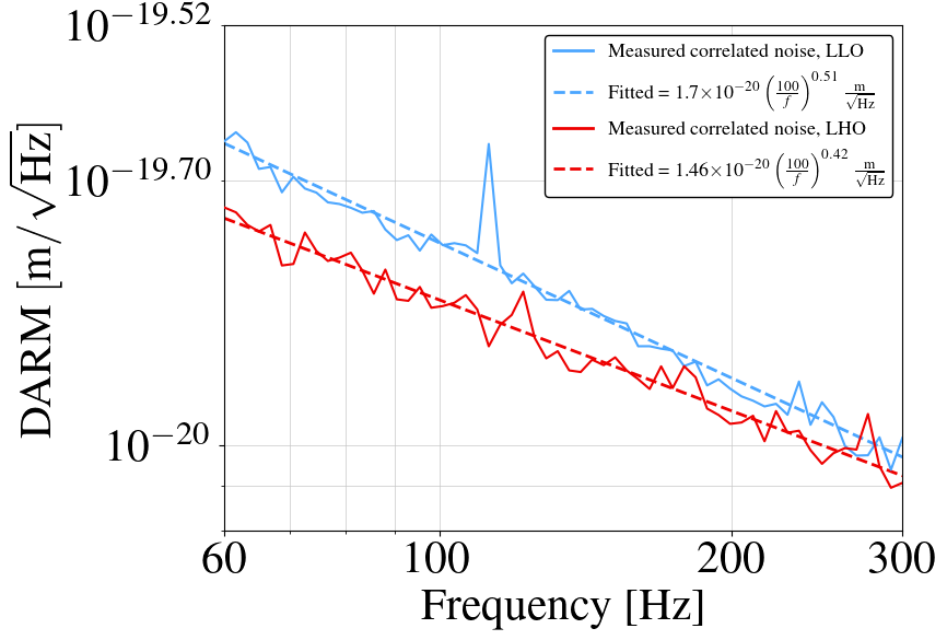
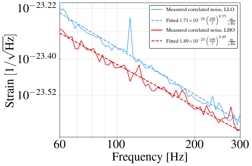
def S_thermal(budget, Phihighn, Phihighn_slope):
    ifo = budget.ifo
    freq = budget.freq

    ifo.Materials.Coating.Phihighn = Phihighn
    ifo.Materials.Coating.Phihighn_slope = Phihighn_slope

    trace = budget.run(freq=freq)

    S_total = S_AMD(freq) + trace.CoatingBrownian.psd + trace.SuspensionThermal.psd + trace.CoatingThermoOptic.psd + trace.SubstrateBrownian.psd + trace.SubstrateThermoElastic.psd


    return S_total


def reportCTN(budget):
    freq = np.geomspace(100,1000,2)
    ifo = budget.ifo
    trace = budget.run(freq=freq)

    ctn = np.sqrt(trace.CoatingBrownian.psd)*L_arm

    slope = np.log10(ctn[1]/ctn[0])
    # print(ctn[0])
    # print(slope)
    return [ctn[0], slope]


# L1 xcorr

f_bin = np.geomspace(60, 300, 60)

budget = gwinc.load_budget('aLIGO')
budget.freq = f_bin


xcorr = lib.DARM('../data/xcorr_budget/1022_Unsqz.h5')
# unsqz = deepcopy(xcorr)
# unsqz.removeLines('DARM'); unsqz.removeLines('CAL');
# unsqz.rebin_log(np.geomspace(10, 5000, 750))

xcorr.S = xcorr.S_xcorr
xcorr.removeLines('DARM'); # xcorr.removeLines('CAL');
xcorr.rebin_log(f_bin)


l1ctn, pcov = scipy.optimize.curve_fit(S_thermal, budget, abs(xcorr.S), p0=[3.9e-4, 0.1])


budget.ifo.Materials.Coating.Phihighn = l1ctn[0]
budget.ifo.Materials.Coating.Phihighn_slope = l1ctn[1]

l1_thermal = deepcopy(budget)

[ctn100Hz, slope] = reportCTN(l1_thermal)
slope = abs(slope)

plt.loglog(f_bin, np.sqrt(abs(xcorr.S)), '-', c=[75/255,166/255,255/255], lw=1.5, zorder=10, label='Measured correlated noise, LLO')
plt.loglog(f_bin, np.sqrt(S_thermal(budget, *l1ctn)), c=[75/255,166/255,255/255], ls='--', lw=2.0,
           label='Fitted  '+str((ctn100Hz*1e20).round(2)) + r'$\times 10^{-20}\left(\frac{100}{f}\right)^{' + str(slope.round(2)) +r'}$ $\frac{\mathrm{m}}{\sqrt{\mathrm{Hz}}}$')


# H1 xcorr

psd = lib.DARM()
psd.f = h1nb_xcorr['Freq'][:]
key = '/budget/CorrelatedDARMMeasured'
psd.S = h1nb_xcorr['CorrelatedDARM'+key+'/PSD'][:]/L_arm**2
# S_calLines = h1nb_xcorr['CorrelatedDARM']['budget']['CalLines']['PSD'][:]
# psd.S -= S_calLines/L_arm**2
# psd.S[(psd.f >= 78.5) & (psd.f <= 79.5)] = np.nan


psd.S[(psd.f >= 53) & (psd.f <= 54)] = np.nan
psd.S[(psd.f >= 77.5) & (psd.f <= 78)] = np.nan
psd.S[(psd.f >= 101.5) & (psd.f <= 102.5)] = np.nan
psd.S[(psd.f >= 270.5) & (psd.f <= 271.5)] = np.nan
psd.S[(psd.f >= 279) & (psd.f <= 280)] = np.nan
psd.S[(psd.f >= 283.5) & (psd.f <= 284.5)] = np.nan
psd.S[(psd.f >= 299) & (psd.f <= 300)] = np.nan
psd.S[(psd.f >= 302) & (psd.f <= 303.5)] = np.nan


psd.removeLines('DARM'); # psd.removeLines('CAL')
psd.setZeroErr(); psd.rebin_log2log(f_bin)


h1ctn, pcov = scipy.optimize.curve_fit(S_thermal, budget, abs(psd.S), p0=[3.9e-4, 0.1])


budget.ifo.Materials.Coating.Phihighn = h1ctn[0]
budget.ifo.Materials.Coating.Phihighn_slope = h1ctn[1]

h1_thermal = deepcopy(budget)
[ctn100Hz, slope] = reportCTN(h1_thermal)
slope = abs(slope)

plt.loglog(f_bin, np.sqrt(abs(psd.S)), '-', c=[238/255,0/255,0/255], lw=1.5, zorder=10, label='Measured correlated noise, LHO')
plt.loglog(f_bin, np.sqrt(S_thermal(budget, *h1ctn)), c=[238/255,0/255,0/255], ls='--', lw=2.0,
           label='Fitted  '+str((ctn100Hz*1e20).round(2)) + r'$\times 10^{-20}\left(\frac{100}{f}\right)^{' + str(slope.round(2)) +r'}$ $\frac{\mathrm{m}}{\sqrt{\mathrm{Hz}}}$')


plt.xlabel('Frequency [Hz]')
plt.ylabel(r'Strain $\mathrm{[1/\sqrt{Hz}]}$')
# plt.title('(b) LIGO Livingston Observatory', fontsize=16)

# plt.xticks([10,20,50,100,200,500,1000,2000,5000], ('10','20','50','100','200','500','1000','2000','5000'))
plt.xticks([60,100,200,300,400], ('60','100','200','300','400'))

plt.xlim(f_bin[0], f_bin[-1])
# plt.ylim(0.8e-20, 3e-20)

grayrgb = 200
plt.grid(True, which='both', color=[grayrgb/255,grayrgb/255,grayrgb/255], linestyle='-', linewidth=0.5)


# legend = plt.legend([handles[idx] for idx in order],[labels[idx] for idx in order], fontsize=13*fontscale, edgecolor='black', ncol=3)
legend = plt.legend(loc='upper right', fontsize=13, edgecolor='black', ncol=1, handlelength=2, markerscale=1)
for line in legend.get_lines(): line.set_linewidth(2)
legend.bbox_to_anchor=(0.5, 1.25)
# legend = ax.legend(edgecolor="black", fontsize=10)
legend.set_zorder(1000)
legend.get_frame().set_alpha(None)
legend.get_frame().set_facecolor('white')


plt.gcf().set_size_inches(8, 6)


# plt.savefig('CTN_fit.svg', bbox_inches='tight')
# plt.savefig('CTN_fit.pdf', bbox_inches='tight')
plt.show()
import scipy.io as io


matplotlib.rc('font',**{'family':'serif','serif':['Times'], 'size':18})
matplotlib.rc('lines',**{'lw':3,'ls':'--'})


file = io.loadmat('../data/thermal/l1nbws_nov23.mat')
ff   = file['ff']
ff = ff.reshape(len(ff))

darm = file['darm']


trace = ctn_budget.run(freq=ff)
total = S_AMD(ff) + trace.CoatingBrownian.psd + trace.SuspensionThermal.psd + trace.CoatingThermoOptic.psd + trace.SubstrateBrownian.psd + trace.SubstrateThermoElastic.psd


# trace = l1_thermal.run(freq=ff)

cto = trace.CoatingThermoOptic.asd
amd = np.sqrt(S_AMD(ff))
sus = trace.SuspensionThermal.asd
sub = np.sqrt(trace.SubstrateBrownian.psd + trace.SubstrateThermoElastic.psd)

# total = np.sqrt(ctn_fit**2 + cto**2 + amd**2 + sus**2 + sub**2)  # with fitted ctn

trace = ctn_budget.run(freq=ff)
ctn = trace.CoatingBrownian.asd
total = np.sqrt(ctn**2 + cto**2 + amd**2 + sus**2 + sub**2)  # with plain ctn


fig, ax = plt.subplots()
ax.loglog(ff, darm, c=[75/255,166/255,255/255],  ls='-', lw=2, zorder=0, label='Measured noise, LLO')
# ax.loglog(ff, total, c=[216/255,54/255,54/255], ls='-', label='Total thermal noise, fit')
# ax.loglog(ff, ctn_fit, c='green', ls=':', label='Coating Brownian, fit')
ax.loglog(ff, total, c=[216/255,54/255,54/255], ls='-', label='Total thermal')
ax.loglog(ff, ctn, c='green',  label='Coating Brownian, witness sample')
ax.loglog(ff, cto, c='#02ccfe',label='Coating thermo-optic')
ax.loglog(ff, amd, c='magenta',label='Acoustic mode dampers')
ax.loglog(ff, sub, c='#fb7d07',label='Substrate (Brownian + thermo-elastic)')
ax.loglog(ff, sus, c='purple', label='Suspension (Brownian)', zorder=0)


plt.xticks([10,20,50,100,200,500,1000,2000,5000], ('10','20','50','100','200','500','1000','2000','5000'))
plt.xlim(10,5000)
plt.ylim(1e-25, 1e-21)
plt.grid(which='major', color='xkcd:grey', alpha=0.3, ls='-')
plt.grid(which='minor', color='xkcd:grey', alpha=0.3, ls=':')

legend = plt.legend(loc='best', fontsize=14, edgecolor='black', handlelength=1.8, labelspacing=.5,)
for line in legend.get_lines(): line.set_linewidth(3)
legend.set_zorder(1000)
legend.get_frame().set_alpha(None)
legend.get_frame().set_facecolor('white')

plt.xlabel('Frequency [Hz]')
plt.ylabel(r'Strain $\mathrm{[1/\sqrt{Hz}]}$')

plt.gcf().set_size_inches(8, 6)

plt.savefig('Thermal_subbudget.svg',bbox_inches='tight')
plt.savefig('Thermal_subbudget.pdf',bbox_inches='tight')

plt.show()
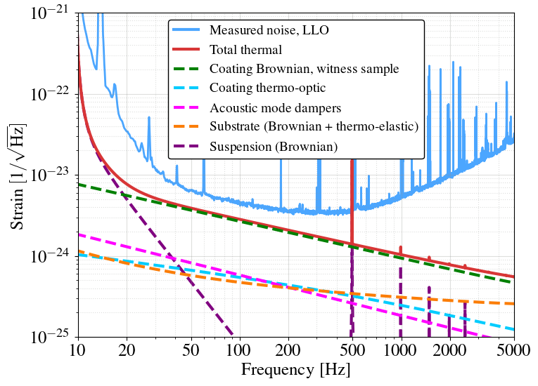
Range plot
#!/usr/bin/env python3
# -*- coding: utf-8 -*-
#
# IFO ranges during chosen time period
# Based on:
# O3a_Range.ipynb by G. Vajente (2020)
# get_range_single_O3b,range_utils by A. Urban,D. Davis,Z. Doctor,M. J. Williams (2021)
# Modified by R. Poggiani (2021, 2022)
# Modified by D. Davis (2024)
# Code is now easier to customize for specific use cases


import numpy as np
from numpy import *
import os
import glob
import time
import sys
import h5py as h5

import gwpy
from gwpy.time import tconvert
from gwpy.timeseries import TimeSeries, TimeSeriesList, TimeSeriesDict
from gwpy.segments import SegmentList, DataQualityDict
# import matplotlib
# matplotlib.use('agg')
# matplotlib.rcParams['text.usetex'] = True
# matplotlib.rcParams['font.family'] = 'STIXGeneral'
# matplotlib.rcParams['font.size'] = 9
# matplotlib.rcParams['savefig.dpi'] = 300
# matplotlib.rcParams['text.latex.preamble'] = r'\usepackage{amsmath}'
# matplotlib.rcParams['legend.fontsize'] = 9


from pylab import *
from matplotlib.colors import LogNorm
from matplotlib import pyplot as plt
plt.rc('axes', axisbelow=True)

def save_fig(fig_id, figure, tight_layout=True):
    path = fig_id + '.png'
    print('Saving figure', fig_id)
    if tight_layout:
        figure.tight_layout()
    figure.savefig(path, format='png', dpi=100)

def save_fig_pdf(fig_id, tight_layout=True):
    path = fig_id + '.pdf'
    print('Saving figure', fig_id)
    if tight_layout:
        plt.tight_layout()
    plt.savefig(path, format='pdf', dpi=100)


def get_range_data(source, channels, start_time, end_time, frametype=None):
    print(start_time, end_time)
    try: # read from source first
        print(f'Trying to read from {source}...')
        data = TimeSeriesDict.read(source, channels=channels,
                start=start_time, end=end_time, pad=0, verbose=True)
    except: # fetch data from NDS2
        try:
            print(f'Trying to read from NDS2 all at once...')
            data = TimeSeriesDict.fetch(channels=channels,
                    start=start_time, end=end_time, pad=0, verbose=True)
        except:
            print(f'Trying to read from NDS2 one by one...')
            data = TimeSeriesDict()
            for chan in channels:
                data[chan] = TimeSeries.get(chan,
                    start=start_time, end=end_time, pad=0, verbose=True)
    return data

def get_segments_data(source, flags, start_time, end_time):
    try: # read from source first
        print(f'Trying to read from {source}...')
        segments = DataQualityDict.read(source, flags)
    except: # fetch data from segments database
        print(f'Trying to read from segments database...')
        segments = DataQualityDict.query_dqsegdb(flags,
                start_time, end_time)
    return segments

def mask_non_observing(data, segments_dict):
    for chan in data.keys():
        for seg in segments_dict.keys():
            if chan[:2] == seg[:2]: # matching channel and segment names
                start_chan = data[chan].t0.value
                end_chan = start_chan + data[chan].duration.value
                full_time = SegmentList([[start_chan, end_chan]])
                mask_times = full_time - segments_dict[seg].active
                data[chan] = data[chan].mask(mask_times)
    return data

def calculate_medians(data, step_size):
    median_data = TimeSeriesDict()
    for chan in data.keys():
        factor = int(step_size / data[chan].dt.value)
        if factor != 1:
            #range_data = repeat(median(range_lho.reshape(-1,factor), axis=1, keepdims=True), factor, axis=1).reshape(-1,1)
            median_data[chan] = median(data[chan].reshape(-1,factor), axis=1)
            median_data[chan].dt = median_data[chan].dt * factor
        else:
            median_data[chan] = data[chan]
    return median_data

# plot labels
ifo_names = {
        'H1': r'$\mathrm{LIGO\  Hanford}$',
        'L1': r'$\mathrm{LIGO\  Livingston}$',
        'V1': r'$\mathrm{Virgo}$',
        'K1': r'$\mathrm{KAGRA}$',
}

colors = {'L1':'#4ba6ff','H1':'#ee0000','V1':'#9b59b6', 'V1pre': '#e5d4ec','V1post':'#b482c8'}

range_labels = {}

# =============== START OF VARIABLES - EDIT BELOW THIS LINE ===============

# imgpath = '../../images/'
imgpath = './'
img_label = 'O4'

# GPS times of start and end of O4a run
gps_start = 1368975618
gps_end = 1389456018
#gps_end = gps_start + (70*86400)
print(gps_start, gps_end)
channels = ['H1:DMT-SNSC_EFFECTIVE_RANGE_MPC.mean', 'L1:DMT-SNSC_EFFECTIVE_RANGE_MPC.mean']
flags = ['H1:DMT-ANALYSIS_READY:1', 'L1:DMT-ANALYSIS_READY:1']
step_size = 3600 # 1 hour

data_file = '../data/range/O4/range_data-%d-%d.gwf'%(gps_start, gps_end-gps_start)
segments_file = '../data/range/O4/segments-%d-%d.xml'%(gps_start, gps_end-gps_start)


#plot params
bins = 80
max_val = 200
min_val = 50

# add month labels?
months = True

# past run markers

# O1 median ranges for H1,L1 from plot_o1.py,based on https://git.ligo.org/agata.trovato/gwosc_data_paper/-/tree/master/range_from_Duncan/O1 with zeros removed
range_labels['O1'] = {
        'H1': 76,
        'L1': 66,
}

# O2 median ranges for H1,L1,V1 from plot_o2.py,based on https://git.ligo.org/agata.trovato/gwosc_data_paper/-/tree/master/range_from_Duncan/O2 with zeros removed
range_labels['O2'] = {
        'H1': 76,
        'L1': 89,
        # 'V1': 28,
}

# O3a median ranges for H1, L1, V1 from GWTC-2 paper, Phys. Rev. X 11 (2021) 021053
range_labels['O3a'] = {
        'H1': 108,
        'L1': 135,
        # 'V1': 45,
}

# O3b median ranges for H1, L1, V1 from GWTC-3 paper
range_labels['O3b'] = {
        'H1': 115,
        'L1': 133,
        # 'V1': 51,
}


# # =============== END OF VARIABLES - DO NOT EDIT BELOW THIS LINE ===============

#### ANALYSIS STARTS HERE

max_date = np.ceil((gps_end - gps_start)/86400)

# set up dicts for later use
ifos = [chan[:2] for chan in channels]
channels_dict = {chan[:2]:chan for chan in channels}
flags_dict = {flag[:2]:flag for flag in flags}

# get data
data = get_range_data(data_file, channels, gps_start, gps_end)
segments = get_segments_data(segments_file, flags, gps_start, gps_end)
data = mask_non_observing(data, segments)
median_data = calculate_medians(data, step_size)

# write out data
if not os.path.isfile(data_file):
    median_data.write(data_file)
else:
    print(f'{data_file} alreadfy exists! Not overwriting...')
if not os.path.isfile(segments_file):
    segments.write(segments_file, format='ligolw')
else:
    print(f'{segments_file} alreadfy exists! Not overwriting...')

# calculate median
run_median = {}
for ifo in ifos:
    run_median[ifo] = np.median(data[channels_dict[ifo]].value[data[channels_dict[ifo]].value > 0.])

# get order to show plots
ifo_order = [i for _, i in sorted(zip(run_median.values(), run_median.keys()))]
ifo_order = ifo_order[::-1]

# make a histogram
run_histo = {}
for ifo in ifos:
    run_histo[ifo], _, _ = plt.hist(median_data[channels_dict[ifo]].value,
        bins = bins, range=(min_val,max_val),
        density=True)

# remove units for easier manipulation
tim_dict = {}
rng_dict = {}
for ifo in ifos:
    tim_dict[ifo] = (median_data[channels_dict[ifo]].times.value - gps_start)/86400
    rng_dict[ifo] = median_data[channels_dict[ifo]].value

range_label_data = []
for run in range_labels.keys():
    for ifo in range_labels[run].keys():
        range_label_data.append([range_labels[run][ifo], range_labels[run][ifo], run, colors[ifo]])

from operator import itemgetter
range_label_data = sorted(range_label_data, key=itemgetter(0,1))
orig_range_label_data = range_label_data.copy()
min_offset = (max_val-min_val)*0.04
min_steps = (max_val-min_val)*0.001
overlap = True
loop = 0
while overlap == True:
    overlap = False
    for i in range(len(range_label_data)-1):
        if abs(range_label_data[i][1] - range_label_data[i+1][1]) < min_offset:
            overlap = True
            # adjust the locations
            range_label_data[i][1] -= min_steps
            range_label_data[i+1][1] += min_steps
    if loop > 1000:
        print('Could not find good locations for the run labels!')
        break
    loop += 1 # to prevent infinite loops
1368975618 1389456018
1368975618 1389456018
Trying to read from ../data/range/O4/range_data-1368975618-20480400.gwf...
Reading (<built-in function format>): |██████████| 1/1 (100%) ETA 00:00
Trying to read from ../data/range/O4/segments-1368975618-20480400.xml...
../data/range/O4/range_data-1368975618-20480400.gwf alreadfy exists! Not overwriting...
../data/range/O4/segments-1368975618-20480400.xml alreadfy exists! Not overwriting...
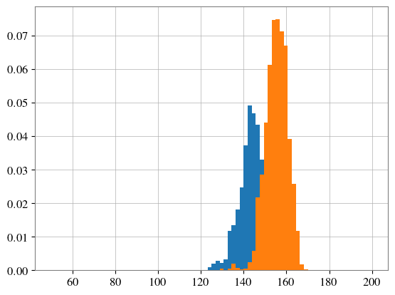
fig, (ax1, ax2) = plt.subplots(1, 2, gridspec_kw={'width_ratios': [2, 1]})
plt.subplots_adjust(wspace=0.12)


lines = {}
for ifo in ifo_order:
    ax1.scatter(tim_dict[ifo], rng_dict[ifo],
            marker='.', s=4,
            label=ifo_names[ifo],
            alpha=1, color=colors[ifo])
    lines[ifo], = plot([0], [0],
            ls='-', linewidth=3,
            label=ifo_names[ifo], color=colors[ifo])

# Marks for beginning of months
from datetime import datetime, timedelta
from dateutil.relativedelta import relativedelta
from calendar import month_abbr
start_date = tconvert(gps_start)
c = 0 - start_date.day
current_date = start_date.replace(day=1)
while c < max_date:
    if c > 0:
        ax1.vlines(c,max_val, max_val-(max_val-min_val)*0.02, color='k', linewidth=1, linestyle='-')
        ax1.text(c-(max_date*0.03),max_val+(max_val-min_val)*0.03, r'$\mathrm{%s}$'%month_abbr[(current_date.month)], color='k', fontsize=12)
    new_date = current_date + relativedelta(months=1)
    c += (new_date - current_date).days
    current_date = new_date

# Marks for median ranges
for label in range_label_data:
    if label[0] < max_val and label[0] > min_val:
        ax1.plot(max_date,label[0],marker=8,color=label[3],markersize=4,linestyle='')
        ax1.text(max_date*1.01,label[1]-(max_val-min_val)*0.02, r'$\mathrm{%s}$'%label[2], color=label[3], fontsize=9)
ax1.set_xlim([0, max_date])
ax1.set_ylim([min_val, max_val])
ax1.set_xlabel(r'$\mathrm{Time\ [days]\ from\ %d\ %s\ %d}$'%(start_date.day, month_abbr[(start_date.month)], start_date.year))
ax1.set_ylabel(r'$\mathrm{Binary\ neutron\ star\ range}\,\mathrm{[Mpc]}$')
ax1.grid(True, which='both')
legend = ax1.legend(handles=([lines[k] for k in lines.keys()]), ncol=1, fontsize=10,edgecolor='black',loc='lower left')
legend.set_zorder(1000)
legend.get_frame().set_alpha(None)
legend.get_frame().set_facecolor('white')


ax2.hist(rng_dict['L1'], color=colors['L1'], bins=30, density=True, histtype='bar', alpha=0.5, orientation='horizontal')
ax2.hlines(run_median['L1'], 0, 0.08, color=colors['L1'], zorder=10, linewidth=1.5, linestyle='--')
ax2.hist(rng_dict['H1'], color=colors['H1'], bins=30, density=True, histtype='bar', alpha=0.5, zorder=20, orientation='horizontal')
ax2.hlines(run_median['H1'], 0, 0.08, color=colors['H1'], linewidth=1.5, linestyle='--')


# Marks for median ranges
for label in range_label_data:
    if label[0] < max_val and label[0] > min_val:
        ax2.plot(0,label[0],marker=9,color=label[3],markersize=4,linestyle='')
        # ax2.text(max_date*1.01,label[1]-(max_val-min_val)*0.02, r'$\mathrm{%s}$'%label[2], color=label[3], fontsize=7)

ax2.set_xlim([0, 0.08])
ax2.set_ylim([min_val, max_val])
ax2.set_xlabel(r'$\mathrm{Probability \ density}$')
ax2.set_ylabel(r'$\mathrm{Binary\ neutron\ star\ range}\,\mathrm{[Mpc]}$')
ax2.grid(True, which='both')
ax2.set_xticks([0,0.02,0.04,0.06,0.08])
# ax2.set_xticklabels(['0', '2', '4', '6', '8'])
ax2.yaxis.tick_right()
ax2.yaxis.set_label_position("right")
ax2.set_yticks([66,76,89,108,115,133, round(run_median['H1']), round(run_median['L1'])])
# ax2.set_yticklabels([])

plt.savefig('range.svg')
plt.savefig('range.pdf')
plt.show()
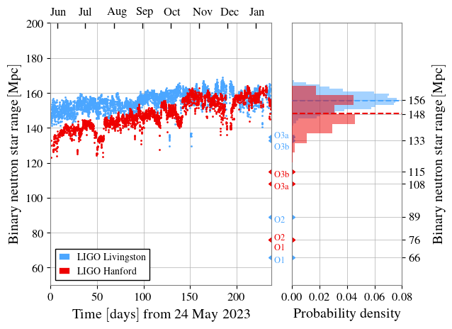
### PLOTTING STARTS HERE

# plot_range_data
fig = plt.figure(figsize=(3.375,3))
ax = fig.gca()
lines = {}
for ifo in ifo_order:
    ax.scatter(tim_dict[ifo], rng_dict[ifo],
            marker='.', s=4,
            label=ifo_names[ifo],
            alpha=1, color=colors[ifo])
    lines[ifo], = plot([0], [0],
            ls='-', linewidth=3,
            label=ifo_names[ifo], color=colors[ifo])

# Marks for beginning of months
from datetime import datetime, timedelta
from dateutil.relativedelta import relativedelta
from calendar import month_abbr
start_date = tconvert(gps_start)
c = 0 - start_date.day
current_date = start_date.replace(day=1)
while c < max_date:
    if c > 0:
        ax.vlines(c,max_val, max_val-(max_val-min_val)*0.02, color='k', linewidth=1, linestyle='-')
        ax.text(c-(max_date*0.03),max_val+(max_val-min_val)*0.03, r'$\mathrm{%s}$'%month_abbr[(current_date.month)], color='k', fontsize=7)
    new_date = current_date + relativedelta(months=1)
    c += (new_date - current_date).days
    current_date = new_date

# Marks for median ranges
for label in range_label_data:
    if label[0] < max_val and label[0] > min_val:
        ax.plot(max_date,label[0],marker=8,color=label[3],markersize=4,linestyle='')
        ax.text(max_date*1.01,label[1]-(max_val-min_val)*0.02, r'$\mathrm{%s}$'%label[2], color=label[3], fontsize=7)
ax.set_xlim([0, max_date])
ax.set_ylim([min_val, max_val])
ax.set_xlabel(r'$\mathrm{Time\ [days]\ from\ %d\ %s\ %d}$'%(start_date.day, month_abbr[(start_date.month)], start_date.year))
ax.set_ylabel(r'$\mathrm{Binary\ neutron\ star\ range}\,\mathrm{[Mpc]}$')
ax.grid(False)
ax.legend(handles=([lines[k] for k in lines.keys()]), ncol=3, fontsize=6,frameon=False,bbox_to_anchor=(0.05,0.95),loc='upper left')
# save_fig_pdf(imgpath+img_label+'_range_hourly_median', figure)


# range histograms with caret markers for median ranges
b = linspace(min_val, max_val, bins+1)
fig = plt.figure(figsize=(3.375,3))
ax = fig.gca()
hist_max = 0
for ifo in ifo_order:
    ax.fill(0.5*(b[1:]+b[:-1]), run_histo[ifo]   / sum(run_histo[ifo])   / (b[1]-b[0]), alpha=0.7, label=ifo_names[ifo], color=colors[ifo])
    hist_max = max([hist_max, max(run_histo[ifo] / sum(run_histo[ifo]) / (b[1]-b[0]))])
i = 0
for ifo in ifo_order:
    ax.vlines(run_median[ifo], 0, hist_max, color=colors[ifo], linewidth=1.5, linestyle='--')
    ax.text(run_median[ifo]-(max_val-min_val)*0.075,   hist_max*(1.05+0.1*i) , '%d Mpc' % round(run_median[ifo]), color=colors[ifo], fontsize=9)
    i += 1

plot_max = hist_max * 1.75

# redo label location finder
min_offset = (max_val-min_val)*0.06
min_steps = (max_val-min_val)*0.001
overlap = True
loop = 0
range_label_data = orig_range_label_data
while overlap == True:
    overlap = False
    for i in range(len(range_label_data)-1):
        if abs(range_label_data[i][1] - range_label_data[i+1][1])*4/len(range_label_data[i][2]+range_label_data[i+1][2]) < min_offset:
            overlap = True
            # adjust the locations
            range_label_data[i][1] -= min_steps
            range_label_data[i+1][1] += min_steps
    if loop > 1000:
        print('Could not find good locations for the run labels!')
        break
    loop += 1 # to prevent infinite loops

# run markers
for label in range_label_data:
    if label[0] < max_val and label[0] > min_val:
        ax.plot(label[0],plot_max, marker=11,color=label[3],markersize=4,linestyle='')
        ax.text(label[1]-(max_val-min_val)*0.04, plot_max*1.02, r'$\mathrm{%s}$'%label[2], color=label[3], fontsize=5)
ax.grid(False)
ax.legend(loc='upper left', ncol=2,fontsize=7,columnspacing=0.5,frameon=False, bbox_to_anchor=(0., 0.95))
ax.set_ylim([0, plot_max])
ax.set_xlim([min_val, max_val])
ax.set_xlabel(r'$\mathrm{Binary\ neutron\ star\ range}\,\mathrm{[Mpc]}$')
ax.set_ylabel(r'$\mathrm{Probability\ density}$')
# save_fig_pdf(imgpath+img_label+'_range_histograms')
Text(0, 0.5, '$\\mathrm{Probability\\ density}$')
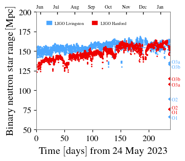
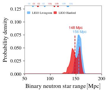
VT plot
from datetime import datetime, timedelta, date
from dateutil.relativedelta import relativedelta
from calendar import month_abbr


matplotlib.rc('font',**{'family':'serif','serif':['Times'], 'size':16})

previous_gw_events = [20150914,20151012,20151226,
    20170104,20170608,20170729,20170809,20170814,20170817,20170818,20170823,
    20190408,20190412,20190421,20190425,20190426,
    20190503,20190510,20190512,20190513,20190517,20190519,20190521,20190521,
    20190602,20190630,20190701,20190706,20190707,
    20190718,20190720,20190727,20190728,
    20190814,20190828,20190828,20190901,20190910,
    20190910,20190915,20190923,20190924,
    20190930,
    20191105,20191109,20191129,20191204,
    20191204,20191205,20191213,20191215,20191216,20191222,
    20200105,20200112,20200114,20200115,
    20200128,20200129,20200208,20200213,
    20200219,20200224,20200225,20200302,
    20200311,20200316];

O4a_list = [
    20230529,20230601,20230605,20230606,20230608,20230609,20230624,20230627,
    20230628,20230630,20230630,20230702,20230704,20230706,20230707,20230708,
    20230708,20230708,20230709,20230723,20230726,20230729,20230731,20230802,
    20230805,20230806,20230807,20230811,20230814,20230814,20230819,20230820,
    20230822,20230824,20230825,20230831,20230904,20230911,20230914,20230919,
    20230920,20230922,20230922,20230924,20230927,20230927,20230928,20230930,
    20231001,20231005,20231005,20231008,20231014,20231020,20231020,20231028,
    20231029,20231102,20231104,20231108,20231110,20231113,20231113,20231114,
    20231118,20231118,20231118,20231119,20231123,20231127,20231129,20231206,
    20231206,20231213,20231223,20231224,20231226,20231231,20240104,20240107,
    20240109];

O4b_list = [
    20240413, 20240421, 20240422, 20240426, 20240426, 20240428, 20240430,
    20240501, 20240505, 20240507, 20240511, 20240512, 20240513, 20240514,
    20240514, 20240515, 20240520, 20240525, 20240527, 20240527, 20240530,
    20240531, 20240601, 20240601, 20240615, 20240615, 20240618, 20240621,
    20240621, 20240621, 20240622, 20240627, 20240629, 20240630, 20240703,
    20240705, 20240716, 20240807, 20240813, 20240813, 20240825, 20240830,
    20240902, 20240907, 20240908, 20240908, 20240910, 20240915, 20240915,
    20240916, 20240917, 20240919, 20240920, 20240920, 20240921, 20240922,
    20240923, 20240924, 20240925, 20240930, 20240930, 20241002, 20241006,
    20241007, 20241009, 20241009, 20241009, 20241011]


gw_event = previous_gw_events + O4a_list + O4b_list;

datetime_event = []
for j in range(len(gw_event)):
    time = str(gw_event[j])
    yyyy = int(time[0:4])
    mm = int(time[4:6])
    dd = int(time[6:])
    datetime_event.append(date(yyyy,mm,dd))

num_event = len(gw_event);


O1_start  = date(2015,9,12);
O1_end    = date(2016,1,19);
len_O1    = O1_end - O1_start;

O2_start  = date(2016,11,30);
O2_end    = date(2017,8,25);
len_O2    = O2_end - O2_start;

O3a_start = date(2019,4,1);
O3a_end   = date(2019,10,1);
len_O3a   = O3a_end - O3a_start;


O3b_start = date(2019,11,1);
O3b_end   = date(2020,3,26); # BTL changed to covid end
len_O3b   = O3b_end - O3b_start;

O4a_start = date(2023,5,24);
O4a_end   = date(2024,1,16);
len_O4a   = O4a_end - O4a_start;

O4b_start = date(2024,  4, 10)
O4b_end   = date(2024,  10,  11) # updated on June 2024
len_O4b   = O4b_end - O4b_start


total_days = len_O1 + len_O2 + len_O3a + len_O3b + len_O4a + len_O4b;
O1  = len_O1.days;
O2  = (len_O1 + len_O2).days;
O3a = (len_O1 + len_O2 + len_O3a).days;
O3b = (len_O1 + len_O2 + len_O3a + len_O3b).days;
O4a = (len_O1 + len_O2 + len_O3a + len_O3b + len_O4a).days;
O4b = (len_O1 + len_O2 + len_O3a + len_O3b + len_O4a + len_O4b).days;

nev_O1 = 3;
nev_O2 = 8;
nev_O3a = 32;
nev_O3b = 24;
nev_O1_O3 = nev_O1 + nev_O2 + nev_O3a + nev_O3b;
nev_O4a   = len(O4a_list)
nev_O1_O4a = nev_O1 + nev_O2 + nev_O3a + nev_O3b + nev_O4a
nev_O4b   = num_event - nev_O1_O4a


event_days = []
for i in range(num_event):
    if (datetime_event[i]>=O1_start and datetime_event[i]<=O1_end):
        event_days.append((datetime_event[i]-O1_start).days);
    elif (datetime_event[i]>=O2_start and datetime_event[i]<=O2_end):
        event_days.append((datetime_event[i]-O2_start+len_O1).days)
    elif (datetime_event[i]>=O3a_start and datetime_event[i]<=O3a_end):
        event_days.append((datetime_event[i]-O3a_start+len_O1+len_O2).days)
    elif (datetime_event[i]>=O3b_start and datetime_event[i]<=O3b_end):
        event_days.append((datetime_event[i]-O3b_start+len_O1+len_O2+len_O3a).days)
    elif (datetime_event[i]>=O4a_start and datetime_event[i]<=O4a_end):
        event_days.append((datetime_event[i]-O4a_start+len_O1+len_O2+len_O3a+len_O3b).days)
    elif (datetime_event[i]>=O4b_start and datetime_event[i]<=O4b_end):
        event_days.append((datetime_event[i]-O4b_start+len_O1+len_O2+len_O3a+len_O3b+len_O4a).days)

# event_days.append(1000) # for plotting purposes

O4_start = nev_O1_O3 + 1;
# % O4 events are still "significant events" and not GW events, as of Dec 2023
# %%
cumu = np.linspace(1,num_event,num_event);

ymax = 220
facealpha = 1.0


filly1 = np.array([ymax,ymax])
filly2 = np.array([0,0])

# fig, ax = plt.subplot()
plt.fill_between([0,O1], filly1, where=filly1>filly2, fc=[0.9, 0.7, 0.7], alpha=facealpha, ec='black',lw=0.5)
plt.fill_between([O1, O2], filly1, where=filly1>filly2, fc=[0.7, 0.9, 0.7], alpha=facealpha, ec='black',lw=0.5)
plt.fill_between([O2, O3a], filly1, where=filly1>filly2, fc=[0.7, 0.7, 0.9], alpha=facealpha, ec='black',lw=0.5)
plt.fill_between([O3a, O3b], filly1, where=filly1>filly2, fc=[0.8, 0.7, 1.0], alpha=facealpha, ec='black',lw=0.5)
plt.fill_between([O3b, O4a], filly1, where=filly1>filly2, fc=[0.95, 0.9, 0.0], alpha=facealpha, ec='black',lw=0.5)
plt.fill_between([O4a, O4b], filly1, where=filly1>filly2, fc='wheat', alpha=facealpha, ec='black',lw=0.5)


text_height=0.7
plt.text(O1/2, ymax*text_height, 'O1', horizontalalignment='center', verticalalignment='center')
plt.text((O1+O2)/2, ymax*text_height, 'O2', horizontalalignment='center', verticalalignment='center')
plt.text((O2+O3a)/2, ymax*text_height, 'O3a', horizontalalignment='center', verticalalignment='center')
plt.text((O3a+O3b)/2, ymax*text_height, 'O3b', horizontalalignment='center', verticalalignment='center')
plt.text((O3b+O4a)/2, ymax*text_height, 'O4a', horizontalalignment='center', verticalalignment='center')
plt.text((O4a+O4b)/2, ymax*text_height, 'O4b*', horizontalalignment='center', verticalalignment='center')


plt.xlim(0, total_days.days)
plt.ylim(0, ymax)


slopeO3 = (nev_O3a+nev_O3b)/(O3b-O2)
# plt.plot([O2,O3b],[nev_O1+nev_O2,nev_O1+nev_O2+nev_O3a+nev_O3b], ls='--', color='gray', lw=2)
plt.plot([O2,O4b],[nev_O1+nev_O2, nev_O1+nev_O2 + slopeO3*(O4b-O2)], ls='--', color='gray', lw=2)
# plt.plot([O2,O4a],[nev_O1+nev_O2, nev_O1+nev_O2], ls='--', color='gray', lw=2)

slopeO4 = (num_event - (nev_O1+nev_O2+nev_O3a+nev_O3b))/225
# plt.plot([O3b,O4a],[nev_O1+nev_O2+nev_O3a+nev_O3b, nev_O1+nev_O2+nev_O3a+nev_O3b+slopeO4*(O4a-O3b)], ls='--', color='black', lw=2)

plt.step(event_days, cumu, color='gray', lw=1.5);
# % redraw the O4 events in grey
plt.step(event_days[nev_O1_O3:], cumu[nev_O1_O3:], color='black', lw=1.5);


# tt=title({['O1+O2+O3 = ' num2str(nev_O1_O3),', O4a* = ' num2str(nev_O4a), ', Total = ' num2str(num_event)]});

plt.xlabel('Time (Days)', fontsize=16);
plt.ylabel('Cumulative Detections/Candidates', fontsize=16);


# set(gca,'FontSize', fontsize-2, 'FontWeight','bold','LineWidth', 1.5);
# xx = get(gca,'xlim');
# yy = get(gca,'ylim');
# credit_y_offset = 0.1;
# text(xx(2)*1.03, yy(1)-credit_y_offset*yy(2), 'Credit: LIGO-Virgo-KAGRA Collaboration', 'Color', 'k',
#     'FontSize', 12, 'FontAngle', 'italic','horizontalalignment','right');

# %%% document number %%%
# text(xx(1), yy(1)-credit_y_offset*yy(2), 'LIGO-G2302098-v11', 'Color', 'k', 'FontSize', 12, 'FontAngle', 'italic');
# %%%%%%%%%%%%%%%%%%%%%%%

plt.grid(False)
# %text(xx(1),yy(2),' * O4a entries are preliminary candidates found online.','verticalalignment','top', 'FontSize', 14)
# text(xx(1)+200,yy(2)*0+195,' * O4a entries are preliminary candidates found online.','verticalalignment','top', 'FontSize', 20)

ax1 = plt.gca()
ax2 = ax1.secondary_xaxis("top")
ax2.set_xticks([0,O1,O2,O3a,O3b,O4a])

ax3 = ax1.secondary_yaxis("right")
ax3.set_yticks([nev_O1,nev_O1+nev_O2,nev_O1+nev_O2+nev_O3a,
                nev_O1+nev_O2+nev_O3a+nev_O3b,nev_O1+nev_O2+nev_O3a+nev_O3b+nev_O4a,num_event])


plt.gcf().set_size_inches(7, 6)
plt.savefig('cumu.svg')
plt.savefig('cumu.pdf')

plt.show()
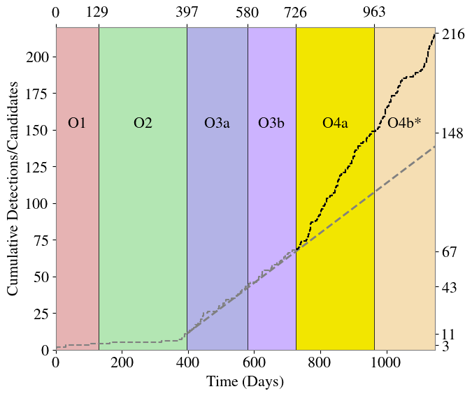
Damping noise
import numpy as np
import matplotlib
import matplotlib.pyplot as plt
import scipy.io as io
import seaborn as sea

# matplotlib.use('agg')
# matplotlib.rcParams['text.usetex'] = True
# matplotlib.rcParams['font.size'] = 12
# matplotlib.rcParams['savefig.dpi'] = 300
# matplotlib.rcParams['text.latex.preamble'] = r'\usepackage{amsmath}'
# matplotlib.rcParams['legend.fontsize'] = 12


# sea.set_palette('colorblind')


## Set up plot
dot = 1   # 1 is dense, 10 is sparsely distributed dots
plt.rc('font',**{'family':'serif','serif':['Times'], 'size':16})
plt.rc('text', usetex=True)
plt.rc('axes', **{'grid':True,'grid.which':'both'})
plt.rc('lines', **{'linestyle':(0,(1,dot)),'lw':2})
# plt.rc('lines', **{'linestyle':'','linewidth':.1,'marker':'o','markersize':2,'markeredgecolor':'none'})


# load LLO data from .mat file

data = io.loadmat('../data/damping/DampNBdata.mat')

keys = {'quadnoise', 'bsnoise', 'triplenoise'}

idx_bs  = np.where(data['bsnoise'] !=0)[0]
bsnoise = data['bsnoise'][idx_bs]
f_bs = data['f_bs'][idx_bs]

idx_triple = np.where(data['triplenoise'] !=0)[0]
triplenoise = data['triplenoise'][idx_triple]
f_triple = data['f_triple'][idx_triple]

idx_quad  = np.where(data['quadnoise'] !=0)[0]
quadnoise = data['quadnoise'][idx_quad]
f_quad = data['f_quad'][idx_quad]


dot = 0.8   # 1 is dense, 10 is sparsely distributed dots

fig, ax = plt.subplots()
ax.loglog(data['f_darm'], data['darm'], ls='-', c=[75/255,166/255,255/255], linewidth=2, label='Measured noise, LLO')
ax.loglog(data['f_sum'], data['allnoise'], ls='-', c=[189/255,189/255,50/255], linewidth=2, label='Suspension damping \n(quads+triples)')
ax.loglog(f_quad, quadnoise, c='darkorange', zorder=1000, ls=(0,(1,dot)), lw=2, label='Quadruple suspensions')
ax.loglog(f_bs, bsnoise, c='limegreen', ls=(0,(1,dot)), lw=2, label='Beamsplitter suspension')
ax.loglog(f_triple, triplenoise, c='darkorchid', ls=(0,(1,dot)), lw=2, label='Triple suspensions')


legend = plt.legend(loc='upper right', edgecolor='black', fontsize=13, handlelength=1.5, markerscale=3)
for line in legend.get_lines(): line.set_linewidth(3)
legend.set_zorder(1000)
legend.get_frame().set_alpha(None)
legend.get_frame().set_facecolor('white')

plt.xticks(list(np.arange(10,31,1)),
           ('10','', '12','','14', '','16','','18', '', '20','', '22', '','24','', '26','','28','','30'))

ax.set_xlim(10, 30)
ax.set_ylim(1e-25, 1e-20)


ax.grid(which='both', color='grey', ls=':', alpha= 0.3)
ax.set_xlabel('Frequency [Hz]',)
plt.ylabel(r'Strain $\mathrm{[1/\sqrt{Hz}]}$')


plt.gcf().set_size_inches(7, 5)
plt.savefig('DampingNoise.svg', bbox_inches='tight')
plt.savefig('DampingNoise.pdf', bbox_inches='tight')

plt.show()
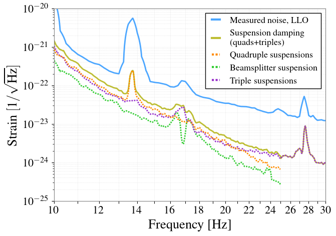
ASC budget
import numpy as np
import matplotlib
import matplotlib.pyplot as plt
import h5py
import seaborn as sea

# matplotlib.use('agg')
# matplotlib.rcParams['text.usetex'] = True
# matplotlib.rcParams['font.size'] = 12
# matplotlib.rcParams['savefig.dpi'] = 300
# matplotlib.rcParams['text.latex.preamble'] = r'\usepackage{amsmath}'
# matplotlib.rcParams['legend.fontsize'] = 12


## Set up plot
dot = 1   # 1 is dense, 10 is sparsely distributed dots
plt.rc('font',**{'family':'serif','serif':['Times'], 'size':16})
plt.rc('text', usetex=True)
plt.rc('axes', **{'grid':True,'grid.which':'both'})
plt.rc('lines', **{'linestyle':(0,(1,dot)),'linewidth':2,'marker':'none','markersize':8,'markeredgecolor':'none'})
# plt.rc('lines', **{'linestyle':'','linewidth':.1,'marker':'o','markersize':2,'markeredgecolor':'none'})


freq = h1nb['Freq'][:]
total_asc = np.sqrt(h1nb['H1']['budget']['ASC']['PSD'][:])
ch_p = np.sqrt(h1nb['H1']['budget']['ASC']['budget']['CHARDPit']['PSD'][:])
dh_p = np.sqrt(h1nb['H1']['budget']['ASC']['budget']['DHARDPit']['PSD'][:])
dh_y = np.sqrt(h1nb['H1']['budget']['ASC']['budget']['DHARDYaw']['PSD'][:])
ch_y = np.sqrt(h1nb['H1']['budget']['ASC']['budget']['CHARDYaw']['PSD'][:])
cs_p = np.sqrt(h1nb['H1']['budget']['ASC']['budget']['CSOFTPit']['PSD'][:])


# darm = np.sqrt(h1nb['H1/budget/DARMMeasured/PSD'][:])
ffs = np.linspace(1,100,1000)
darm = np.interp(ffs, h1nb['Freq'], np.sqrt(h1nb['H1/budget/DARMMeasured/PSD']))

# remove injection notches, zeros, etc
total_asc[(freq >= 13) & (freq <= 15) & (total_asc/L_arm<1e-22)] = np.nan
total_asc[(freq >= 15) & (freq <= 18) & (total_asc/L_arm<1e-23)] = np.nan
total_asc[(freq >= 25) & (freq <= 35) & (total_asc/L_arm<1e-24)] = np.nan
total_asc[total_asc/L_arm<1e-25] = np.nan


# %%
fig, ax = plt.subplots(figsize=(12,8))
ax.loglog(ffs, darm/L_arm, c=[238/255,0/255,0/255], ls='-', marker='none', lw=2, label='Measured noise, LHO')
ax.loglog(freq, total_asc/L_arm, c=[214/255,40/255,40/255], ls='-', label='Alignment control', lw=1.5, alpha=0.6, zorder=0)
# ax.loglog(freq, total_asc/L_arm, c='slategrey', ls='-', label='Alignment control', lw=2, alpha=0.7, zorder=0)
ax.loglog(freq, ch_p/L_arm, c='magenta', label='Common axis, pitch', alpha=0.9)
ax.loglog(freq, ch_y/L_arm, c='yellowgreen', label='Common axis, yaw', zorder=100)
ax.loglog(freq, dh_p/L_arm, c='royalblue',  label='Differential axis, pitch', alpha=0.9)
ax.loglog(freq, dh_y/L_arm, c='purple', label='Differential axis, yaw', zorder=101)  #'#1f77b4'


ax.set_xlim(10, 60)
ax.set_ylim(1e-25, 1e-20)
ax.grid(which='both', color='grey', ls=':', alpha= 0.3)

ax.set_xticks([10, 20, 30, 40, 50, 60])
ax.set_xticklabels([10, 20, 30, 40, 50, 60])
ax.set_xlabel('Frequency [Hz]')
ax.set_ylabel(r'Strain $\mathrm{[1/\sqrt{Hz}]}$')

legend = plt.legend(loc='best', edgecolor='black', fontsize=13, handlelength=1.5, markerscale=3)
for line in legend.get_lines(): line.set_linewidth(3)
legend.set_zorder(1000)
legend.get_frame().set_alpha(None)
legend.get_frame().set_facecolor('white')


plt.gcf().set_size_inches(7, 5)
plt.savefig('ASC_budget_plot.svg',bbox_inches='tight')
plt.savefig('ASC_budget_plot.pdf',bbox_inches='tight')
plt.show()
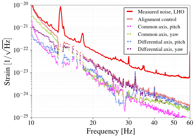
Laser noise budget
dot = 1   # 1 is dense, 10 is sparsely distributed dots
lw1 = 2.0  # model curve
lw2 = 2.0  # measured curve
traces = {                              # color,                 linestyle, linewidth, zorder, lgdorder, label
    '/budget/DARMMeasured':             [[238/255,0/255,0/255]    ,         '-', 1.0,  10,  1, 'Measured noise, LHO'],
    # '':                                 [[0/255,0/255,0/255]      ,         '-', 1.0, 100,  2, 'Sum of known noises'],
    # '/budget/Quantum':                  [[146/255,104/255,173/255],        '--', lw1, 15,  3, 'Quantum'],
    # '/budget/Thermal':                  [[216/255,54/255,54/255]  ,        '--', lw1, 16,  4, 'Thermal'],
    # '/budget/ResidualGas':              [[189/255,189/255,50/255] ,        '--', lw1, 17,  5, 'Residual gas'],
    # '/budget/Seismic':                  [[43/255,160/255,72/255]  , (0,(1,dot)), lw2, 30,  6, 'Seismic'],
    # '/budget/Newtonian':                [[33/255,191/255,207/255] ,         '-', 1.0,  5,  7, 'Newtonian'],
    # '/budget/LSC':                      [[245/255,126/255,32/255] , (0,(1,dot)), lw2, 40,  8, 'Auxiliary length control'],
    # '/budget/ASC':                      [[214/255,40/255,40/255]  , (0,(1,dot)), lw2, 50,  9, 'Alignment control'],
    '/budget/Laser/budget/InputJitter': ['blue',                      (0,(1,dot)), lw2, 50, 10, 'Beam jitter'], #[32/255,119/255,180/255]
    '/budget/Laser/budget/Intensity':   [[43/255,160/255,72/255]  ,   (0,(1,dot)), lw2,  5, 12, 'Laser intensity'], # neg w/ freq noise
    '/budget/Laser/budget/Frequency':   [[214/255,121/255,177/255],   (0,(1,dot)), lw2, 20, 13, 'Laser frequency'],
    # '/budget/Dark':                     [[147/255,149/255,152/255], (0,(1,dot)), lw2, 50, 14, 'Photodetector dark'],
    # '/budget/OMCLength':                [[0/255,0/255,0/255]      , (0,(1,dot)), lw2, 50, 15, 'Output mode cleaner length'],
    # '/budget/PUMDAC':                   [[141/255,88/255,77/255]  , (0,(1,dot)), lw2, 50, 16, 'Penultimate-mass actuator'],
    # '/budget/OSEM':                                        ['cyan', (0,(1,dot)), lw2, 50, 17, 'Suspension damping (quad)'],
}

plt.rcdefaults()
matplotlib.rc('font',**{'family':'serif','serif':['Times'], 'size':16})
matplotlib.rc('text', usetex=True)


freq = np.geomspace(10,5000,1500)

S_total = h1nb['Freq'][:]*0
# S_total = freq*0

Slist = []

for key in traces:
    psd = lib.DARM()
    psd.f = h1nb['Freq'][:]
    psd.S = h1nb['H1'+key+'/PSD'][:]/L_arm**2

    fmt = traces[key]

    lgdorder = fmt[4]
    # if lgdorder > 5:
    #     psd.setZeroErr(); psd.rebin_log2log(freq)

    if key == '/budget/DARMMeasured':
        plt.loglog(psd.f, np.sqrt(psd.S), c=fmt[0], ls=fmt[1], lw=fmt[2], zorder=fmt[3], label=fmt[5])
    else:
        Slist.append(psd.S)
        S_total += psd.S


psd = lib.DARM()
psd.f = h1nb['Freq'][:]
psd.S = S_total
psd.setZeroErr(); psd.rebin_log2log(freq)
plt.loglog(psd.f, psd.S**0.5, c='black', alpha=0.9, ls='-', lw=1, zorder=100, label='Sum of laser noises')


# j = 0
# for key in traces:
#     fmt = traces[key]
#     if key != '/budget/DARMMeasured':
#         # plt.loglog(psd.f, np.sqrt(Slist[j]), c=fmt[0], ls=fmt[1], lw=fmt[2], zorder=fmt[3], label=fmt[5])
#         plt.loglog(psd.f, np.sqrt(Slist[j]), c=fmt[0], ls='', lw=fmt[2], zorder=fmt[3], label=fmt[5], marker='o',markersize=2.5,alpha=1)
#         j += 1
for key in traces:
    psd = lib.DARM()
    psd.f = h1nb['Freq'][:]
    psd.S = h1nb['H1'+key+'/PSD'][:]/L_arm**2

    # remove injection notches, zeros, etc
    psd.S[psd.S < 1e-70] = np.nan

    fmt = traces[key]
    if lgdorder > 5:
        psd.setZeroErr(); psd.rebin_log2log(freq)

    if key != '/budget/DARMMeasured':
        # plt.loglog(psd.f, psd.S**0.5, c=fmt[0], ls=fmt[1], lw=fmt[2], zorder=fmt[3], label=fmt[5])
        plt.loglog(psd.f, psd.S**0.5, c=fmt[0], ls='', lw=fmt[2], zorder=fmt[3], label=fmt[5], marker='o',markersize=2.5,alpha=1)


plt.xlabel('Frequency [Hz]')
plt.ylabel(r'Strain $\mathrm{[1/\sqrt{Hz}]}$')
# plt.title('(a) LIGO Hanford Observatory (LHO)', fontsize=16)

plt.xticks([10,20,50,100,200,500,1000,2000,5000], ('10','20','50','100','200','500','1000','2000','5000'))
plt.xlim(20, 5000)
plt.ylim(1e-25, 1e-22)

grayrgb = 200
plt.grid(True, which='both', color=[grayrgb/255,grayrgb/255,grayrgb/255], linestyle=':', linewidth=0.5)


# legend = plt.legend([handles[idx] for idx in order],[labels[idx] for idx in order], fontsize=13*fontscale, edgecolor='black', ncol=3)
legend = plt.legend(loc='upper center', fontsize=14, edgecolor='black', ncol=1, markerscale=2.5, handlelength=1.5)
for line in legend.get_lines(): line.set_linewidth(2.5)
legend.set_zorder(1000)
legend.get_frame().set_alpha(None)
legend.get_frame().set_facecolor('white')


plt.gcf().set_size_inches(10, 5)

plt.savefig('H1_laser_budget.svg', bbox_inches='tight')
plt.savefig('H1_laser_budget.pdf', bbox_inches='tight')
plt.show()
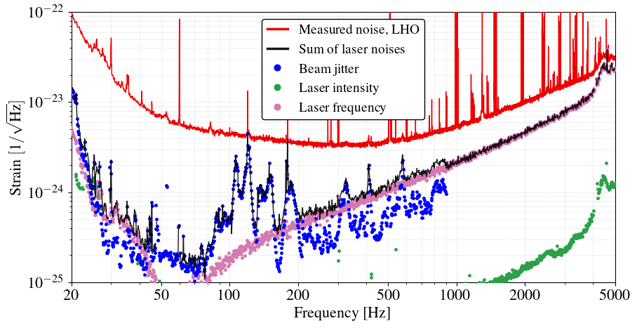
dot = 1   # 1 is dense, 10 is sparsely distributed dots
lw1 = 2.0  # model curve
lw2 = 2.0  # measured curve
traces = {                              # color,                 linestyle, linewidth, zorder, lgdorder, label
    '/budget/DARMMeasured':             [[75/255,166/255,255/255]    ,         '-', 1.0,  10,  1, 'Measured noise, LLO'],
    # '':                                 [[0/255,0/255,0/255]      ,         '-', 1.0, 100,  2, 'Sum of known noises'],
    # '/budget/Quantum':                  [[146/255,104/255,173/255],        '--', lw1, 15,  3, 'Quantum'],
    # '/budget/Thermal':                  [[216/255,54/255,54/255]  ,        '--', lw1, 16,  4, 'Thermal'],
    # '/budget/ResidualGas':              [[189/255,189/255,50/255] ,        '--', lw1, 17,  5, 'Residual gas'],
    # '/budget/Seismic':                  [[43/255,160/255,72/255]  , (0,(1,dot)), lw2, 30,  6, 'Seismic'],
    # '/budget/Newtonian':                [[33/255,191/255,207/255] ,         '-', 1.0, 5,  7, 'Newtonian'],
    # '/budget/LSC':                      [[245/255,126/255,32/255] , (0,(1,dot)), lw2, 40,  8, 'Auxiliary length control'],
    # '/budget/ASC':                      [[214/255,40/255,40/255]  , (0,(1,dot)), lw2, 50,  9, 'Alignment control'],
    '/budget/Laser/budget/InputJitter': ['blue' , (0,(1,dot)), lw2, 50, 10, 'Beam jitter'],
    '/budget/Laser/budget/Intensity':   [[43/255,160/255,72/255]  , (0,(1,dot)), lw2, 5, 12, 'Laser intensity'], # neg w/ freq noise
    '/budget/Laser/budget/Frequency':   [[214/255,121/255,177/255], (0,(1,dot)), lw2, 50, 13, 'Laser frequency'],
    # '/budget/Dark':                     [[147/255,149/255,152/255], (0,(1,dot)), lw2, 50, 14, 'Photodetector dark'],
    # '/budget/OMCLength':                [[0/255,0/255,0/255]      , (0,(1,dot)), lw2, 50, 15, 'Output mode cleaner length'],
    # '/budget/PUMDAC':                   [[141/255,88/255,77/255]  , (0,(1,dot)), lw2, 50, 16, 'Penultimate-mass actuator'],
    # '/budget/OSEM':                                        ['cyan', (0,(1,dot)), lw2, 50, 17, 'Suspension damping (quad)'],
}


matplotlib.rc('font',**{'family':'serif','serif':['Times'], 'size':16})
matplotlib.rc('text', usetex=True)


# freq = np.geomspace(10,5000,400)
freq = np.geomspace(10,5000,1500)

# for name, data in h1nb['H1/budget'].items():
#     plt.loglog(freq, np.sqrt(data['PSD'][:])/L_arm, label=name)

# S_total = l1nb['Freq'][:]*0
S_total = freq*0

Slist = []

for key in traces:
    psd = lib.DARM()
    psd.f = l1nb['Freq'][:]
    psd.S = l1nb['L1'+key+'/PSD'][:]/L_arm**2
    # psd.S = abs(psd.S)

    fmt = traces[key]

    lgdorder = fmt[4]

    if lgdorder > 5:
        psd.setZeroErr(); psd.rebin_log2log(freq)
        S_total += psd.S

    if key == '/budget/DARMMeasured':
        plt.loglog(psd.f, np.sqrt(psd.S), c=fmt[0], ls=fmt[1], lw=fmt[2], zorder=fmt[3], label=fmt[5])
    else:
        Slist.append(psd.S)


plt.loglog(psd.f, np.sqrt(S_total), ls='-', c='black', alpha=0.9, lw=1., zorder=100, label='Sum of laser noises')


j = 0
for key in traces:
    fmt = traces[key]
    if key == '/budget/DARMMeasured':
        donothing=1
    else:
        # plt.loglog(psd.f, np.sqrt(Slist[j]), c=fmt[0], ls=fmt[1], lw=fmt[2], zorder=fmt[3], label=fmt[5])
        plt.loglog(psd.f, np.sqrt(Slist[j]), c=fmt[0], ls='', lw=fmt[2], zorder=fmt[3], label=fmt[5], marker='o',markersize=2.5,alpha=1)
        j += 1


plt.xlabel('Frequency [Hz]')
plt.ylabel(r'Strain $\mathrm{[1/\sqrt{Hz}]}$')
# plt.title('(b) LIGO Livingston Observatory (LLO)', fontsize=16)

plt.xticks([10,20,50,100,200,500,1000,2000,5000], ('10','20','50','100','200','500','1000','2000','5000'))
plt.xlim(20, 5000)
plt.ylim(1e-25, 1e-22)


grayrgb = 200
plt.grid(True, which='both', color=[grayrgb/255,grayrgb/255,grayrgb/255], linestyle=':', linewidth=0.5)


# legend = plt.legend([handles[idx] for idx in order],[labels[idx] for idx in order], fontsize=13*fontscale, edgecolor='black', ncol=3)
legend = plt.legend(loc='upper center', fontsize=14, edgecolor='black', ncol=1, markerscale=2.5, handlelength=1.5)
for line in legend.get_lines(): line.set_linewidth(2.5)
legend.set_zorder(1000)
legend.get_frame().set_alpha(None)
legend.get_frame().set_facecolor('white')


plt.gcf().set_size_inches(10, 5)


plt.savefig('L1_laser_budget.svg', bbox_inches='tight')
plt.savefig('L1_laser_budget.pdf', bbox_inches='tight')
plt.show()
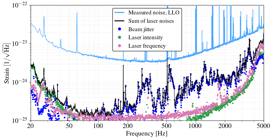
MICH feedforward
import numpy as np
import matplotlib
import matplotlib.pyplot as plt
import h5py
import seaborn as sea


#preshaping function
data = np.loadtxt('../data/LSC/michff_tf.txt')
freq = data[:,0]
shaping = data[:,1] + 1j*data[:,2]

# no ff data
data = np.loadtxt('../data/LSC/MICH_no_ff_TF.txt')
freq1 = data[:,0]
MICH_noff = data[:,1] + 1j*data[:,2]

# first ff tuning data
data = np.loadtxt('../data/LSC/ff_before_iterative.txt')
MICH_ff_before_iter = data[:,1] + 1j*data[:,2]

# second ff tuning data
data = np.loadtxt('../data/LSC/ff_after_iterative.txt')
MICH_ff_after_iter = data[:,1] + 1j*data[:,2]

# darm no mich ff
data = np.loadtxt('../data/LSC/CALIB_STRAIN_NOLINES_MICH_DEC18_FF_ON.txt')
freq_on = data[:,0]
darm_on = data[:,1]*L_arm

#darm w/ mich ff
data = np.loadtxt('../data/LSC/CALIB_STRAIN_NOLINES_MICH_DEC18.txt')
freq_off = data[:,0]
darm_off = data[:,1]*L_arm

# adjust freq vectors and data length
idx = freq1 <= freq.max()

freq1 = freq1[idx]
MICH_noff = MICH_noff[idx]
MICH_ff_before_iter = MICH_ff_before_iter[idx]
MICH_ff_after_iter = MICH_ff_after_iter[idx]
darm_on = darm_on[idx]
darm_off = darm_off[idx]

# %%
# calculating MICH contribution from TF data
MICH_off =  darm_off / np.abs(MICH_noff/shaping)

MICH_before = darm_on * np.abs(MICH_ff_before_iter/shaping)

MICH_after = darm_on * np.abs(MICH_ff_after_iter/shaping)


# %%
# fig, ax = plt.subplots(figsize=(12,8))
# plt.loglog(freq1, darm_on/L_arm, ls='-', lw=1, c=[238/255,0/255,0/255], label='Measured noise')
# plt.loglog(freq1, darm_off/L_arm, ls=(0,(2,dot)), lw=1.0, c=[238/255,0/255,0/255], label='Measured noise, No feedforward')
# plt.loglog(freq1, MICH_off/L_arm, ls=(0,(2,dot)), lw=1.0, c='xkcd:blue grey', label='MICH length, No feedforward')
# plt.loglog(freq1, MICH_before/L_arm, ls='-', lw=1, c='xkcd:blue grey', label='MICH length, 1st tuning')
# plt.loglog(freq1, MICH_after/L_arm, ls='-', lw=1, c='xkcd:navy', label='MICH length, 2nd tuning')

# in displacement units:
plt.loglog(freq1, darm_on, ls='-', lw=1, c=[238/255,0/255,0/255], label='DARM')
plt.loglog(freq1, darm_off, ls=(0,(2,dot)), alpha=0.6, lw=1.0, c=[238/255,0/255,0/255], label='DARM (No MICH feedforward)')
plt.loglog(freq1, MICH_off, ls=(0,(2,dot)), lw=1.0, c='xkcd:blue grey', label='MICH\ \ (No MICH feedforward)')
plt.loglog(freq1, MICH_before, ls='-', lw=1, c='xkcd:blue grey', label='MICH (1st tuning)')
plt.loglog(freq1, MICH_after, ls='-', lw=1, c='black', label='MICH (2nd tuning)')

#plt.loglog(MICH_freq, MICH_NB, label='MICH NB')
plt.xlim(10,80)
plt.ylim(1e-23, 1e-17)
# plt.ylim(1e-27, 1e-21)
plt.grid(True, which='both', color='xkcd:grey', alpha= 0.5)


legend = plt.legend(loc='best', fontsize=12, edgecolor='black', ncol=1, handlelength=2)
legend.set_zorder(1000)
legend.get_frame().set_alpha(None)
legend.get_frame().set_facecolor('white')
# change the line width for the legend
for line in legend.get_lines():
    line.set_linewidth(2)


plt.xticks([10, 20, 30, 40, 50, 60, 70, 80], ['10', '20', '30', '40', '50', '60', '70', '80'])
# plt.xticklabels([20, 30, 40, 50, 60])

plt.xlabel('Frequency [Hz]')
# plt.ylabel(r'Strain $\mathrm{[1/\sqrt{Hz}]}$')
plt.ylabel(r'Displacement $\mathrm{[m/\sqrt{Hz}]}$')


plt.gcf().set_size_inches(8, 5)

plt.savefig('MICH_FF_plot.svg', bbox_inches='tight')
plt.savefig('MICH_FF_plot.pdf', bbox_inches='tight')
plt.show()
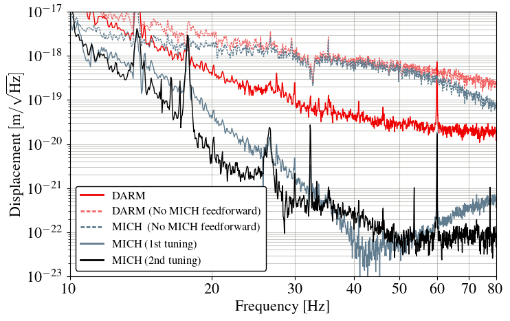
High power challenges
# import warnings
# warnings.filterwarnings('ignore')
# from numpy import *
# import numpy
# %matplotlib inline
# from pylab import *
# from matplotlib.colors import LogNorm
# import os
# import time
# from scipy.signal import *
# import nds2
# import pickle
# import sys
# from tqdm.notebook import tqdm

# from gwpy.time import tconvert

# import gpstime
# import datetime


# data = pickle.load(open('../data/high_power/lowfreqnoise_sub.pickle', 'rb'))
# fr = data['fr']
# channels = list(data['Shh'].keys())

# #sp = data['sp']
# trend = data['trend']

# fr2 = data['fr2']
# Shh = data['Shh']
# Srr = data['Srr']

# gps = array(list(Shh[channels[0]].keys()))
# dates = {g: datetime.datetime.strptime(gpstime.tconvert(g), '%Y-%m-%d %H:%M:%S.%f %Z') for g in gps}

# band = [20, 50]
# idx = (fr2>band[0])*(fr2<band[1])
# blrms_orig = {c:{} for c in channels}
# blrms_sub  = {c:{} for c in channels}

# for g in gps:
#     for c in channels:
#         blrms_orig[c][g] = exp(mean(log(Shh[c][g][idx]))) / exp(mean(log(Shh[c][gps[0]][idx])))
#         blrms_sub[c][g]  = exp(mean(log(Srr[c][g][idx]))) / exp(mean(log(Shh[c][gps[0]][idx])))

# ch = 'H1:CAL-DELTAL_EXTERNAL_DQ'

# # find date on May 1, before DCPD value change
# idx = np.where(np.logical_and(gps>1366934418, gps<1367020818))[0][0]

# end = gps[idx]
# matplotlib.rc('font',**{'family':'serif','serif':['Times'], 'size':16})
# matplotlib.rc('text', usetex=True)


# fig, ax = subplots(2, 1, figsize=(10,12))
# #ax1b = ax[1].twinx()
# for g in gps:
#     l1 = ax[0].plot(dates[g], blrms_orig[ch][g], 'o', color='darkgray', alpha=1, markeredgecolor='none', label='Calibrated differential\narm length')
#     l2 = ax[0].plot(dates[g], blrms_sub[ch][g], 'o', color='orange', alpha=1, markeredgecolor='none', label='With coherence-based\nLSC subtraction')
#     ax[1].plot(dates[g], trend['H1:IMC-PWR_IN_OUT_DQ.mean'][g], 'ko')
#     #ax1b.plot(dates[g], trend['H1:OMC-DCPD_SUM_OUT_DQ.mean'][g], 'ro')

# ax[0].set_ylabel('Normalized Noise %d-%d Hz' % (band[0], band[1]))
# ax[0].set_xlabel('Date')
# ax[1].set_xlabel('Date')
# ax[0].set_ylim([0.3, 3])
# # ax[0].set_title(ch)

# ax[0].set_xlim([dates[gps.min()], dates[end]])

# ax[0].legend(handles=(l1[0],l2[0]))

# ax[1].set_ylim([55,82])
# ax[1].set_ylabel('PSL Input power [W]')

# ax[1].set_xlim([dates[gps.min()], dates[end]])

# #ax1b.set_ylim([15,50])
# #ax1b.set_ylabel('DCPD mean [mA]', color='r')
# #ax1b.tick_params(axis='y', labelcolor='r')

# xticks = arange(dates[gps.min()].date(), dates[end].date()+datetime.timedelta(days=5), datetime.timedelta(days=5))
# for i in range(2):
#     ax[i].set_xticks(xticks)
#     ax[i].set_xticklabels([x.astype(datetime.datetime).strftime('%m/%d') for x in xticks])
#     ax[i].tick_params(axis='x', labelrotation=0, size=6)


# ax[0].grid(True)
# ax[1].grid(True)

# # tight_layout()

# # plt.gcf().set_size_inches(10, 8)

# plt.savefig('LowFreqNoise.svg')
# plt.savefig('LowFreqNoise.pdf')
# plt.show()
Laser frequency noise
data = np.loadtxt('../data/lasernoise/LLO_freq_inloop.txt')
l1_inloopf = data[:,0]
l1_inloop = data[:,1]


data = np.loadtxt('../data/lasernoise/LHO_freq_cp.txt')
l1_f = data[:,0]
l1_rtS = data[:,1]


data = np.loadtxt('../data/lasernoise/LHO_freq_inloop.txt')
h1_inloopf = data[:,0]
h1_inloop = data[:,1]

data = np.loadtxt('../data/lasernoise/LHO_freq_outofloop.txt')
h1_outloopf = data[:,0]
h1_outloop = data[:,1]

data = np.loadtxt('../data/lasernoise/LLO_freq_cp.txt')
h1_f = data[:,0]
h1_rtS = data[:,1]


S_FDS = h1nb['H1/budget/DARMMeasured/PSD'][:]/L_arm**2


# fig, (ax1, ax2, ax3) = plt.subplots(3, 1, gridspec_kw={'height_ratios': [2, 1, 1]})
# fig, (ax1, ax2, ax3) = plt.subplots(3, 1)
# plt.subplots_adjust(hspace=0.05)

matplotlib.rc('font',**{'family':'serif','serif':['Times'], 'size':14})


plt.subplot(3,1,1)
plt.loglog(h1nb['Freq'][:], np.sqrt(S_FDS), ls='-', lw=1, c='black', label='Measured noise, LHO')
plt.loglog(h1_f, h1_rtS, ls='-', lw=1, c=[238/255,0/255,0/255], label='LHO frequency noise projection')
plt.loglog(l1_f, l1_rtS, ls='-', lw=1, c=[75/255,166/255,255/255], label='LLO frequency noise projection')


plt.xlim(10, 5000)
plt.ylim(1e-26, 1e-20)
plt.grid(True, which='both', color='xkcd:grey', alpha= 0.5)

legend = plt.legend(loc='best', fontsize=12, edgecolor='black', ncol=1, handlelength=1.5)
for line in legend.get_lines(): line.set_linewidth(2.5)
legend.bbox_to_anchor=(0.5, 1.25)
# legend = ax.legend(edgecolor="black", fontsize=10)
legend.set_zorder(1000)
legend.get_frame().set_alpha(None)
legend.get_frame().set_facecolor('white')

plt.grid(True, which='both', color='xkcd:grey', alpha= 0.5, ls=':')
plt.xticks([10,20,50,100,200,500,1000,2000,5000], ('10','20','50','100','200','500','1000','2000','5000'))
plt.yticks([1e-26, 1e-25, 1e-24, 1e-23, 1e-22, 1e-21, 1e-20,])


plt.xlabel('Frequency [Hz]')
plt.ylabel(r'Strain $\mathrm{[1/\sqrt{Hz}]}$')


plt.subplot(3,1,2)
plt.loglog(h1_outloopf, h1_outloop, ls='-', lw=1, c='orange', label='LHO frequency noise, out-of-loop')
plt.loglog(h1_inloopf, h1_inloop, ls='-', lw=1, c=[238/255,0/255,0/255], label='LHO frequency noise, in-loop')
plt.loglog(l1_inloopf, l1_inloop, ls='-', lw=1, c=[75/255,166/255,255/255], label='LLO frequency noise, in-loop')


plt.xlim(20,80)
plt.ylim(1e-7, 1e-3)
plt.grid(True, which='both', color='xkcd:grey', alpha= 0.5)
plt.minorticks_on()

legend = plt.legend(loc='best', fontsize=12, edgecolor='black', ncol=1, handlelength=1.5)
for line in legend.get_lines(): line.set_linewidth(2.5)
legend.bbox_to_anchor=(0.5, 1.25)
# legend = ax.legend(edgecolor="black", fontsize=10)
legend.set_zorder(1000)
legend.get_frame().set_alpha(None)
legend.get_frame().set_facecolor('white')

plt.grid(True, which='both', color='xkcd:grey', alpha= 0.5, ls=':')
plt.xticks([10,20,50,100,200,500,1000,2000,5000], ('10','20','50','100','200','500','1000','2000','5000'))
plt.xlim(10, 5000)
plt.yticks([1e-7, 1e-6, 1e-5, 1e-4, 1e-3])

plt.xlabel('Frequency [Hz]')
plt.ylabel(r'Frequency noise $\mathrm{[Hz/\sqrt{Hz}]}$')


plt.subplot(3,1,3)
plt.loglog(h1_inloopf, np.interp(h1_inloopf, h1_f, h1_rtS)/h1_inloop, ls='-', lw=1, c=[238/255,0/255,0/255], label='LHO coupling from frequency noise to strain')
plt.loglog(l1_inloopf, np.interp(l1_inloopf, l1_f, l1_rtS)/l1_inloop, ls='-', lw=1, c=[75/255,166/255,255/255], label='LLO coupling from frequency noise to strain')
# plt.loglog(h1_outloopf, np.interp(h1_outloopf, h1_f, h1_rtS)/h1_outloop)


plt.xlim(10,5000)
plt.ylim(1e-20, 1e-15)
plt.grid(True, which='both', color='xkcd:grey', alpha= 0.5)
plt.minorticks_on()

legend = plt.legend(loc='best', fontsize=12, edgecolor='black', ncol=1, handlelength=1.5)
for line in legend.get_lines(): line.set_linewidth(2.5)
legend.bbox_to_anchor=(0.5, 1.25)
legend.set_zorder(1000)
legend.get_frame().set_alpha(None)
legend.get_frame().set_facecolor('white')

plt.grid(True, which='both', color='xkcd:grey', alpha= 0.5, ls=':')
plt.xticks([10,20,50,100,200,500,1000,2000,5000], ('10','20','50','100','200','500','1000','2000','5000'))
plt.yticks([1e-20, 1e-19, 1e-18, 1e-17, 1e-16, 1e-15])

plt.xlabel('Frequency [Hz]')
plt.ylabel(r'Coupling function $\mathrm{[1/Hz]}$')


# plt.tight_layout()
plt.subplots_adjust(hspace=0.25)
plt.gcf().set_size_inches(7, 10)

plt.savefig('FreqNoise.svg', bbox_inches='tight')
plt.savefig('FreqNoise.pdf', bbox_inches='tight')
plt.show()
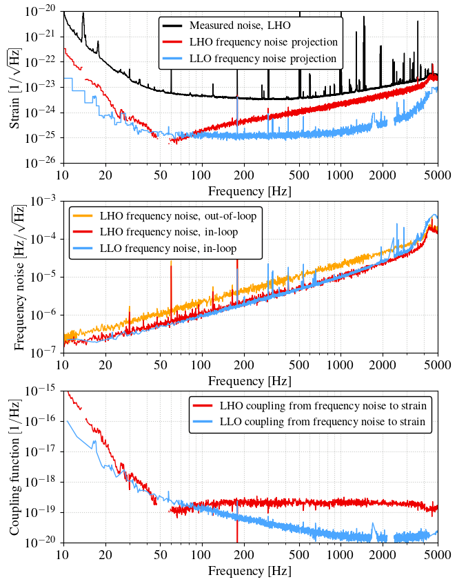
Beam jitter noise
# fig, (ax1, ax2, ax3) = plt.subplots(3, 1, gridspec_kw={'height_ratios': [2, 1]})
# fig, (ax1, ax2, ax3) = plt.subplots(3, 1)
# plt.subplots_adjust(hspace=0.05)

matplotlib.rc('font',**{'family':'serif','serif':['Times'], 'size':14})


data = np.loadtxt('../data/lasernoise/LLO_jitter_wit_pit.txt')
l1_pitwitf = data[:,0]
l1_pitwit = data[:,1]

data = np.loadtxt('../data/lasernoise/LLO_jitter_wit_yaw.txt')
l1_yawwitf = data[:,0]
l1_yawwit = data[:,1]

l1_witf = l1_pitwitf
l1_wit = np.sqrt(l1_pitwit**2 + l1_yawwit**2)


data = np.loadtxt('../data/lasernoise/LLOpit_jitter_cp.txt')
l1_pitf = data[:,0]
l1_pit = data[:,1]

data = np.loadtxt('../data/lasernoise/LLOyaw_jitter_cp.txt')
l1_yawf = data[:,0]
l1_yaw = data[:,1]

l1_cp = np.sqrt(l1_pit**2 + l1_yaw**2)


data = np.loadtxt('../data/lasernoise/LHO_jitter_wit_pit.txt')
h1_pitwitf = data[:,0]
h1_pitwit = data[:,1]

data = np.loadtxt('../data/lasernoise/LHO_jitter_wit_yaw.txt')
h1_yawwitf = data[:,0]
h1_yawwit = data[:,1]

h1_witf = h1_pitwitf
h1_wit = np.sqrt(h1_pitwit**2 + h1_yawwit**2)


data = np.loadtxt('../data/lasernoise/LHOpit_jitter_cp.txt')
h1_pitf = data[:,0]
h1_pit = data[:,1]


data = np.loadtxt('../data/lasernoise/LHOyaw_jitter_cp.txt')
h1_yawf = data[:,0]
h1_yaw = data[:,1]
h1_yaw = np.interp(h1_pitf, h1_yawf, h1_yaw)

h1_cp = np.sqrt(h1_pit**2 + h1_yaw**2)


S_FDS = h1nb['H1/budget/DARMMeasured/PSD'][:]/L_arm**2


plt.subplot(3,1,1)

plt.loglog(h1nb['Freq'][:], np.sqrt(S_FDS), ls='-', lw=1, c='black', label='Measured noise, LHO')
# plt.loglog(h1_pitf, h1_cp*np.interp(h1_pitf, h1_witf, h1_wit), ls='-', lw=1, c=[238/255,0/255,0/255], label='LHO input jitter projection')
plt.loglog(h1_pitf, np.sqrt((h1_pit*np.interp(h1_pitf, h1_pitwitf, h1_pitwit))**2 + (h1_yaw*np.interp(h1_pitf, h1_yawwitf, h1_yawwit))**2),
           ls='-', lw=1, c=[238/255,0/255,0/255], label='LHO input jitter projection')
plt.loglog(l1_pitf, np.sqrt((l1_pit*np.interp(l1_pitf, l1_pitwitf, l1_pitwit))**2 + (l1_yaw*np.interp(l1_pitf, l1_yawwitf, l1_yawwit))**2),
           ls='-', lw=1, c=[75/255,166/255,255/255], label='LLO input jitter projection')
# plt.loglog(l1_pitf, l1_cp*np.interp(l1_pitf, l1_witf, l1_wit), ls='-', lw=1, c=[75/255,166/255,255/255], label='LLO input jitter projection')


plt.xlim(10,1000)
plt.ylim(1e-26, 1e-20)
plt.grid(True, which='both', color='xkcd:grey', alpha= 0.5)

legend = plt.legend(loc='best', fontsize=12, edgecolor='black', ncol=1, handlelength=1.5)
for line in legend.get_lines(): line.set_linewidth(2.5)
legend.bbox_to_anchor=(0.5, 1.25)
# legend = ax.legend(edgecolor="black", fontsize=10)
legend.set_zorder(1000)
legend.get_frame().set_alpha(None)
legend.get_frame().set_facecolor('white')

plt.minorticks_on()
plt.xticks([10,20,50,100,200,500,1000], ('10','20','50','100','200','500','1000'))
plt.yticks([1e-26, 1e-25, 1e-24, 1e-23, 1e-22, 1e-21, 1e-20,]) #, ('10','20','50','100','200','500','1000'))


plt.xlabel('Frequency [Hz]')
plt.ylabel(r'Strain $\mathrm{[1/\sqrt{Hz}]}$')
plt.grid(True, which='both', color='xkcd:grey', alpha= 0.5, ls=':')


RIN_to_jitter_factor_mn = 7433


plt.subplot(3,1,2)
plt.loglog(h1_witf, h1_wit*RIN_to_jitter_factor_mn, ls='-', lw=1, c=[238/255,0/255,0/255], label='LHO beam jitter witness')
plt.loglog(l1_witf, l1_wit*RIN_to_jitter_factor_mn, ls='-', lw=1, c=[75/255,166/255,255/255], label='LLO beam jitter witness')


plt.xlim(10,1000)
# plt.ylim(1e-12, 1e-8)
plt.ylim(1e-8, 1e-4)
plt.grid(True, which='both', color='xkcd:grey', alpha= 0.5)

legend = plt.legend(loc='best', fontsize=12, edgecolor='black', ncol=1, handlelength=1.5)
for line in legend.get_lines(): line.set_linewidth(2.5)
# legend.bbox_to_anchor=(0.5, 1.25)
# legend = ax.legend(edgecolor="black", fontsize=10)
legend.set_zorder(1000)
legend.get_frame().set_alpha(None)
legend.get_frame().set_facecolor('white')


plt.xticks([10,20,50,100,200,500,1000], ('10','20','50','100','200','500','1000'))
plt.yticks([1e-8, 1e-7, 1e-6, 1e-5, 1e-4])

plt.xlabel('Frequency [Hz]')
plt.ylabel(r'Beam jitter noise $\mathrm{[1/\sqrt{Hz}]}$')
plt.grid(True, which='both', color='xkcd:grey', alpha= 0.5, ls=':')


plt.subplot(3,1,3)
plt.loglog(h1_pitf, h1_pit/RIN_to_jitter_factor_mn, ls='-', lw=1, c=[238/255,0/255,0/255], label='LHO, pitch')
plt.loglog(h1_pitf, h1_yaw/RIN_to_jitter_factor_mn, ls='-', lw=1, c='orange', label='LHO, yaw')
plt.loglog(l1_pitf, l1_pit/RIN_to_jitter_factor_mn, ls='-', lw=1, c=[75/255,166/255,255/255], label='LLO, pitch')
plt.loglog(l1_yawf, l1_yaw/RIN_to_jitter_factor_mn, ls='-', lw=1, c=[75/255,166/255/2,255/255], label='LLO, yaw')
# plt.loglog(h1_outloopf, np.interp(h1_outloopf, h1_f, h1_rtS)/h1_outloop)


plt.xlim(10,1000)
plt.ylim(1e-20, 1e-17)
plt.grid(True, which='both', color='xkcd:grey', alpha= 0.5, ls=':')

legend = plt.legend(loc='best', fontsize=12, edgecolor='black', ncol=1, handlelength=1.5)
for line in legend.get_lines(): line.set_linewidth(2.5)
legend.bbox_to_anchor=(0.5, 1.25)
# legend = ax.legend(edgecolor="black", fontsize=10)
legend.set_zorder(1000)
legend.get_frame().set_alpha(None)
legend.get_frame().set_facecolor('white')


plt.xticks([10,20,50,100,200,500,1000], ('10','20','50','100','200','500','1000'))

plt.xlabel('Frequency [Hz]')
plt.ylabel(r'Coupling function (a.u.)')


plt.subplots_adjust(hspace=0.28)
plt.gcf().set_size_inches(7, 10)

plt.savefig('JitterNoise.svg', bbox_inches='tight')
plt.savefig('JitterNoise.pdf', bbox_inches='tight')
plt.show()
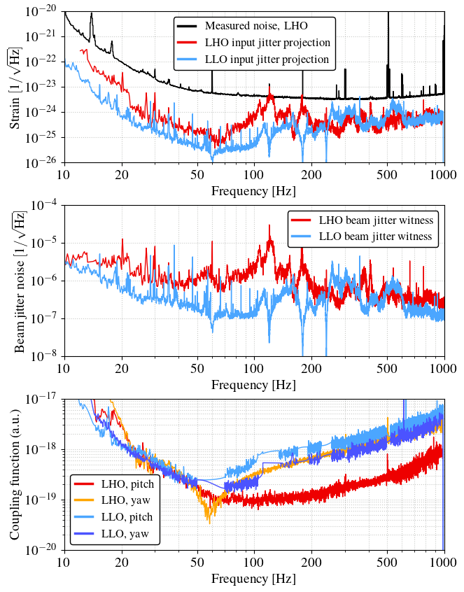
H1 sqz nlg scans
from matplotlib.lines import Line2D


data_dir = '../data/h1_sqz_nlg_scans'  #os.path.join(os.getcwd())
print('using saved txt data from',data_dir)


## Set up plot
plt.rc('font',**{'family':'serif','serif':['Times'], 'size':16})
plt.rc('text', usetex=True)
plt.rc('axes', **{'grid':True,'grid.which':'both'})
plt.rc('lines', **{'linewidth':1.5,'markersize':8,'markeredgecolor':'k'})
plt.rc('legend', **{'fontsize':11,'title_fontsize':11}) #,'labelspacing':0.35,'borderpad':0.4,})


# plot sqz data from text files
sqz_data_fnames = ['NLG_HD_LHO73562_18Oct2023.txt',
                   'NLG_DARM_LHO78025_24May2024.txt',
                   'NLG_DARM_LHO73747_25Oct2023.txt',
                   ]

labels = ['SQZ, -8.0 dB, Homodyne',# 18Oct2023',
          'SQZ, -4.5 dB, Interferometer',# 25Oct2023',
          'SQZ, -4.5 dB, Interferometer',# 'IFO, O4b, lho78025',# 25May2024'
          ]

# # get fit params from npy
# fit_params = np.load(os.path.join(data_dir,'fit_params.npy'))
# fit_params[0][0] = 0.1
# fit_params[1][0] = 0.3

alphas = [0.5, 0.9, 0.9]
mkss = ['*','o','o']
lss = [':','-','-',]


fig,ax = plt.subplots(figsize=(8,5))

for sqz_data_fname, alpha, ls, mks, label in zip(sqz_data_fnames, alphas, lss, mkss, labels):
    print()
    print(sqz_data_fname)

    # load nlg data
    data_fname = os.path.join(data_dir,sqz_data_fname[:-4]+'_data.txt')
    NLG, SQZ, ASQZ, MSQZ = np.loadtxt(data_fname)

    # load nlg fits from above
    fit_fname = os.path.join(data_dir,sqz_data_fname[:-4]+'_fit_calc.txt')
    NLGs, calc_sqz, calc_asqz, calc_msqz = np.loadtxt(fit_fname)

    # plot
    if sqz_data_fname != sqz_data_fnames[-1]:
        plt.plot(NLGs, calc_sqz, 'b', ls=ls, alpha=alpha, ms=0, label='Squeezing ($\phi=0$)')
        plt.plot(NLGs, calc_asqz, 'r', ls=ls, alpha=alpha, ms=0, label='Anti-squeezing ($\phi=\pi/2$)')
        plt.plot(NLGs, calc_msqz, 'g', ls=ls, alpha=alpha, ms=0, label='Mean squeezing ($\phi$ unlocked)')
        #label=f"Loss $\sim$ {(loss*100):0.0f}\%")

    plt.plot(NLG, SQZ,  'b', ls='None', alpha=alpha, marker=mks, zorder=5, label='SQZ')#label=f'SQZ $\sim$ {label[-5:]} dB')
    plt.plot(NLG, MSQZ, 'g', ls='None', alpha=alpha, marker=mks, zorder=5, label='MSQZ')#label=f"MSQZ, Loss $\sim$ {(loss*100):0.0f}\%")
    plt.plot(NLG, ASQZ, 'r', ls='None', alpha=alpha, marker=mks, zorder=5, label='ASQZ')#label='ASQZ')


# access legend objects automatically created from data
handles, labels = plt.gca().get_legend_handles_labels()

# manually make symbols for legend
labels = labels[0:3] + labels[6:9]

bpoint = Line2D([0], [0], label=labels[0], marker=mkss[0], color='b', alpha=alphas[0],
        markeredgecolor='b', markerfacecolor='b', linestyle=lss[0])
rpoint = Line2D([0], [0], label=labels[2], marker=mkss[0], color='r', alpha=alphas[0],
        markeredgecolor='r', markerfacecolor='r', linestyle=lss[0])
gpoint = Line2D([0], [0], label=labels[1], marker=mkss[0], color='g', alpha=alphas[0],
        markeredgecolor='g', markerfacecolor='g', linestyle=lss[0])
bpoint1 = Line2D([0], [0], label=labels[3], marker=mkss[1], color='b', alpha=alphas[1],
        markeredgecolor='k', markerfacecolor='b', linestyle=lss[1])
rpoint1 = Line2D([0], [0], label=labels[4], marker=mkss[1], color='r', alpha=alphas[1],
        markeredgecolor='k', markerfacecolor='r', linestyle=lss[1])
gpoint1 = Line2D([0], [0], label=labels[5], marker=mkss[1], color='g', alpha=alphas[1],
        markeredgecolor='k', markerfacecolor='g', linestyle=lss[1])

# replace legend with manual symbols
handles=[]
handles.extend([bpoint,rpoint,gpoint,bpoint1,rpoint1,gpoint1])

# # with 1 legend
# plt.legend(handles=handles, labels=labels, fontsize=11, ncol=2)

# try it with 2 legends?
legend = plt.legend(handles=handles[0:3], labels=labels[0:3],
                    loc=(0.007, 0.75),
                    title='Homodyne (loss $\sim 10$\%, $\phi_\mathrm{rms}\sim8$ mrad)')
legend.set_zorder(100)
legend.get_frame().set_alpha(0.7)
legend.get_frame().set_facecolor('white')


ax.add_artist(legend)
legend1 = plt.legend(handles=handles[3:], labels=labels[3:],
                     loc=(0.43, 0.75),
                     title='Interferometer (loss $\sim 30$\%, $\phi_\mathrm{rms}\sim22$ mrad)')
legend1.set_zorder(100)
legend1.get_frame().set_alpha(0.7)
legend1.get_frame().set_facecolor('white')

plt.ylabel('Noise relative to no squeezing (dB)',labelpad=-3)
plt.xlabel('Nonlinear gain')
plt.xscale('log')
plt.xlim(0.9,170); plt.ylim(-10,35)
plt.xticks(ticks=[1,10,100],labels=['1','10','100'])

plt.grid(which='major',alpha=0.5,ls='-')
plt.grid(which='minor',alpha=0.5,ls=':')
plt.gcf().set_size_inches(8, 5)

plt.savefig('O4_H1_nlg_hd_ifo.svg', bbox_inches='tight')
plt.savefig('O4_H1_nlg_hd_ifo.pdf', bbox_inches='tight')
using saved txt data from ../data/h1_sqz_nlg_scans

NLG_HD_LHO73562_18Oct2023.txt

NLG_DARM_LHO78025_24May2024.txt

NLG_DARM_LHO73747_25Oct2023.txt
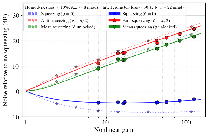
Range as horizon distance / redshift vs mass
#%% From Evan Hall lho70747
import matplotlib as mpl
import numpy as np
import inspiral_range as ir
from matplotlib import pyplot as plt

plt.rcdefaults()
mpl.rc('font',**{'family':'serif','serif':['Times'], 'size':16})
mpl.rc('lines',**{'lw':1})
mpl.rc('text', usetex=True)

def makegrid(ax):
    ax.grid(True, which='major', color='grey', alpha=0.5, ls=':')
    ax.grid(True, which='minor', color='grey', alpha=0.2, ls=':')

text_bbox = dict(fc='w', alpha=0.7, lw=0, pad=0.1)

# %%
fO3_H1, aO3_H1 = np.loadtxt(
    '../data/evan_range_plots/O3-H1-C01_CLEAN_SUB60HZ-1262197260.0_sensitivity_strain_asd_binned.txt',
    unpack=1,
    )
fO3_L1, aO3_L1 = np.loadtxt(
    '../data/evan_range_plots/O3-L1-C01_CLEAN_SUB60HZ-1262141640.0_sensitivity_strain_asd_binned.txt',
    unpack=1,
    )
fO4_H1, aO4_H1 = np.loadtxt(
    '../data/noise_budget/lho_darm_noisebudget_O4a_hotOM2_start1386255618_span1800.txt',
    unpack=1,
    )
aO4_H1 = aO4_H1[(fO4_H1>=10) & (fO4_H1<=5000)]
fO4_H1 = fO4_H1[(fO4_H1>=10) & (fO4_H1<=5000)]

fO4_L1, aO4_L1 = np.loadtxt(
    '../data/noise_budget/L1NB_G2400537_O4a_strain_asd_withSqueezing.txt',
    unpack=1,
    )
fgwinc, agwinc = np.loadtxt(
    '../data/evan_range_plots/gwinc_O4_400kW_4p5dB_FDS.txt',
    unpack=1,
    )

O3_H1_kwargs = dict(
    label='O3, LHO',
    color='red',
    alpha=0.5,
    zorder=25,ls=':',
    )

O3_L1_kwargs = dict(
    label='O3, LLO',
    color='blue',
    alpha=0.5,
    zorder=20,ls=':',
    )


O4_H1_kwargs = dict(
    label='O4, LHO',
    color=[238/255,0/255,0/255],
    alpha=0.9,
    zorder=35,
    )

O4_L1_kwargs = dict(
    label='O4, LLO',
    color=[75/255,166/255,255/255],
    alpha=0.9,
    zorder=30,
    )

gwinc_kwargs = dict(
    label='GWINC (400 kW, 4.5 dB FDS)',
    color='xkcd:blue grey',
    alpha=0.5,
    zorder=5,
    )

O3_H1_dict = dict(
    freq=fO3_H1,
    asd=aO3_H1,
    lw=1,
    kwargs=O3_H1_kwargs,
    )

O3_L1_dict = dict(
    freq=fO3_L1,
    asd=aO3_L1,
    lw=1,
    kwargs=O3_L1_kwargs,
    )

O4_H1_dict = dict(
    freq=fO4_H1,
    asd=aO4_H1,
    lw=1,
    kwargs=O4_H1_kwargs,
    )

O4_L1_dict = dict(
    freq=fO4_L1,
    asd=aO4_L1,
    lw=1,
    kwargs=O4_L1_kwargs,
    )

gwinc400kW_dict = dict(
    freq=fgwinc,
    asd=agwinc,
    lw=1,
    kwargs=gwinc_kwargs
    )

traces_list = [
    O3_L1_dict,
    O3_H1_dict,
    O4_L1_dict,
    O4_H1_dict,
    # gwinc400kW_dict,
    ]


# %%
# Horizon estimates
marr = np.geomspace(1, 2000, 100)

# fig_zhor, ax_zhor = plt.subplots(figsize=(6,4))

fig_zhor, (ax_snr, ax_zhor) = plt.subplots(2, 1, sharex=True,
                                           gridspec_kw={'height_ratios': [1,2.5]})
fig_zhor.set_tight_layout({'pad': 0})
ax_volhor = ax_zhor.twinx()
# fig_volhor, ax_volhor1 = plt.subplots(figsize=(4, 3))

# plot horizon traces
for td in traces_list:
    td['zhor'] = np.zeros_like(marr)
    td['volhor'] = np.zeros_like(marr)
    for i, m in enumerate(marr):
        lal_kwargs = {
        'm1': m/2,
        'm2': m/2,
        #'inclination': np.pi/4,
        'approximant': 'IMRPhenomD',
        }
        td['zhor'][i] = ir.horizon_redshift(td['freq'], td['asd']**2, **lal_kwargs)
        td['volhor'][i] = ir.volume(td['freq'], td['asd']**2, **lal_kwargs) / 1e9
    ax_zhor.loglog(
        marr,
        td['zhor'],
        lw=2,
        **td['kwargs'],
        )
    # ax_volhor.loglog(
    #     marr,
    #     td['volhor'],
    #     lw=2,
    #     **td['kwargs'],
    #     )
# plot ratio traces
for ax in [ax_snr]: #ax_zhor, ax_volhor
    marr_max=1500
    lL1_O4, = ax.loglog(
       marr[marr<marr_max],
       (O4_L1_dict['volhor'] / O3_L1_dict['volhor'])[marr<marr_max],
       lw=1.5,
       ls=(3, (4.5, 1.5,)),
       color=O4_L1_kwargs['color'],
       )
    lH1_O4, = ax.loglog(
        marr[marr<marr_max],
        (O4_H1_dict['volhor'] / O3_H1_dict['volhor'])[marr<marr_max],
        lw=1.5,
        ls=(3, (4.5, 1.5,)),
        color=O4_H1_kwargs['color'],
        )
    print(O4_H1_dict['volhor'][0] / O3_H1_dict['volhor'][0], O4_L1_dict['volhor'][0] / O3_L1_dict['volhor'][0])

# setup plot things nicely
for ax in [ax_zhor]:
    ax.set_xlim([marr[0], 1000])
    ax.set_xlabel(r'Total source-frame mass [$M_\odot$]')
    ax.xaxis.set_major_formatter(mpl.ticker.FuncFormatter(lambda y, _: '{:g}'.format(y)))
    ax.yaxis.set_major_formatter(mpl.ticker.FuncFormatter(lambda y, _: '{:g}'.format(y)))
    ax.text(
        0.035,
        0.93,
        r'SNR threshold = 8',
        ha='left',
        va='top',
        fontsize='small',
        transform=ax.transAxes,
        bbox=text_bbox,
        )
    ax.legend(
        fontsize='x-small',
        handlelength=1.35,
        labelspacing=0.15,
        ).set_zorder(20)
    makegrid(ax)

makegrid(ax_snr)
ax_snr.plot(1,1, color='black', ls='--', lw=2, label='Volume ratio O4 / O3')
ax_snr.set_yscale('log')    # changed upper subplot between log and linear y-scales
ax_snr.set_ylim(1,11)
ax_snr.set_yticks([1,2,5,10],('1','2','5','10'))
ax_snr.set_yticks([3,4,6,7,8,9,],('','','','','','',), minor=True)
ax_snr.minorticks_on()
# ax_snr.xaxis.set_minor_formatter(matplotlib.ticker.NullFormatter())
ax_snr.legend(fontsize=16,loc='upper center',handlelength=1.5,)
ax_snr.set_ylabel('Ratio\nO4 / O3')

h, l = ax_zhor.get_legend_handles_labels()
# h.append(
#     mpl.lines.Line2D([], [], color='xkcd:black', ls=(3, (4.5, 1.5),), lw=2))
# l.append('Volume ratio O4 / O3')
leg_zhor = ax_zhor.legend(
    h,
    l,
    fontsize=16, #'small',
    loc=(0.48,0.035),  # bbox_to_anchor=(0.57, 0),
    handlelength=1.4,
    labelspacing=0.5,
    )
for line in leg_zhor.get_lines(): line.set_linewidth(2.5)
ax_zhor.set_xticks([1, 10, 100, 1000])
ax_zhor.set_yticks([0.01, 0.03, 0.1, 0.3, 1, 3])
ax_zhor.set_ylabel('Horizon redshift')

ax_zhor.set_ylim([00.03, 2])
ax_volhor.set_ylim([0.03, 2])
ax_volhor.set_yscale('log')

right_tick_volhor_targets = np.array([1e-3, 0.1, 10, 30])
tick_idx = [np.argmin(np.abs(td['volhor'] - target)) for target in right_tick_volhor_targets]
ax_volhor.minorticks_off()
ax_volhor.set_yticks(td['zhor'][tick_idx],('0.001','0.1','10','30'))
# ax_volhor.set_yticklabels([f'{val:0.2e}' for val in td['volhor'][tick_idx]])
ax_volhor.set_ylabel('Comoving horizon volume [Gpc$^3$]')

# plt.loglog(td['zhor'], td['volhor'], marker='.')
# plt.loglog(td['zhor'][tick_idx], td['volhor'][tick_idx], marker='o',ls='')
# plt.xlabel('zhor')
# plt.ylabel('volhor')
# plt.grid()

plt.gcf().set_size_inches(6,5)
fig_zhor.savefig('O4_horizon_redshift.pdf', bbox_inches='tight')
# fig_volhor.savefig('O4a_preO4b_comoving_volume.pdf', bbox_inches='tight')
2.4933526148632326 1.8256781640584672
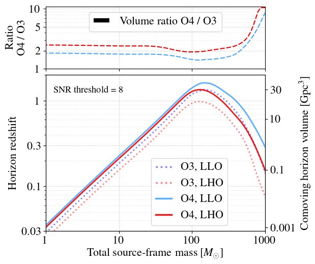
Future filter cavity
D_r = lib.DARM('../data/l1_sqz_1022/1022_Unsqz.h5')
D_s = lib.DARM('../data/l1_sqz_1022/1022_FDS.h5')

# budget = gwinc.load_budget('L1_1022_FC7000.yaml')
budget = gwinc.load_budget("../data/noise_budget/L1_1022_FC7000.yaml")

ifo = budget.ifo
ifo.Squeezer.Type = 'None'
trace = budget.run(freq=D_r.f, ifo=ifo)
C = lib.DARM()
C.f = D_r.f
S_nosqz = trace.Quantum.psd
C.S = D_r.S - S_nosqz


freq = np.geomspace(20,3000,100)

if hasattr(D_s, 'relerrN_n'):
    C.relerr_n = D_s.relerrN_n; C.relerr_p = D_s.relerrN_p
elif hasattr(D_r, 'relerrN_n'):
    C.relerr_n = D_r.relerrN_n; C.relerr_p = D_r.relerrN_p
C.calcErr(); C.removeLines('DARM');
C.rebin_log(freq)

D_r.relerr_n = D_r.relerrD_n; D_r.relerr_p = D_r.relerrD_p
D_r.calcErr(); D_r.removeLines('DARM');
D_r.rebin_log(freq)

D_s.relerr_n = D_s.relerrD_n; D_s.relerr_p = D_s.relerrD_p
D_s.calcErr(); D_s.removeLines('DARM');
D_s.rebin_log(freq)

# trace = budget.run(freq=D_r.f, ifo=ifo)
# M = lib.DARM()
# M.f = D_r.f
# M.S = trace.Quantum.psd
# M.err_n = M.S*np.interp(M.f, np.geomspace(20,2000,100), relerrM_n)
# M.err_p = M.S*np.interp(M.f, np.geomspace(20,2000,100), relerrM_p)

ifo.Squeezer.Type = 'None'
trace = budget.run(freq=freq, ifo=ifo)
S_nosqz = trace.Quantum.psd


Q = D_s - C
# Q.err_n = np.sqrt((D_s.err_n)**2 + (D_r.err_n)**2 + (C.err_n)**2 + (Q.S*np.interp(Q.f, D_s.f_lin, D_s.relerrG_n))**2 + (M.err_n)**2)
# Q.err_p = np.sqrt((D_s.err_p)**2 + (D_r.err_p)**2 + (C.err_p)**2 + (Q.S*np.interp(Q.f, D_s.f_lin, D_s.relerrG_p))**2 + (M.err_p)**2)
Q.err_n = np.sqrt((D_s.err_n)**2 + (D_r.err_n)**2 + (C.err_n)**2 + (Q.S*np.interp(Q.f, D_s.f_lin, D_s.relerrG_n))**2 )
Q.err_p = np.sqrt((D_s.err_p)**2 + (D_r.err_p)**2 + (C.err_p)**2 + (Q.S*np.interp(Q.f, D_s.f_lin, D_s.relerrG_p))**2 )


M_s = lib.DARM(); M_s.f = np.geomspace(20,2000,1000);
ifo.Squeezer.Type = 'Freq Dependent'
trace = budget.run(freq=M_s.f, ifo=ifo)
M_s.S = trace.Quantum.psd
plt.loglog(Q.f, np.sqrt(Q.S))
plt.errorbar(Q.f, np.sqrt(abs(Q.S)), [Q.err_n, Q.err_p]/(2*np.sqrt(abs(Q.S))), marker='o', alpha=0.8,
                 ms=3,ls='-',lw=0, elinewidth=1,capsize=0,mew=0,zorder=10,label='l')


plt.loglog(M_s.f, np.sqrt(M_s.S))
plt.show()
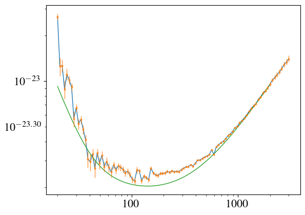
import inspiral_range

def db(num):
    return 20*np.log10(num)

def db2mag(num):
    return 10**(num/20)


c = 3e8; L_FC = 300;
PRXcolor = np.array([173,3,222])/255
sqzcolor = 'mediumorchid'
idealcolor = 'pink'
phasesqz = 13.9


# # budget = gwinc.load_budget('L1_1022_FC7000.yaml')
# budget = gwinc.load_budget("../data/noise_budget/L1_1022_FC7000.yaml")

# ifo = budget.ifo


colors = ['deepskyblue',
         'olive',
         'lime',
         'teal']


ifo.Squeezer.Type = 'None'
trace = budget.run(freq=M_s.f, ifo=ifo)
S_nosqz_long = trace.Quantum.psd


pH_UNS, = plt.plot([20,1000], [0,0], '--', lw=2, c='black', zorder=0)


R1R2 = (1-ifo.Squeezer.FilterCavity.Ti)*(1-ifo.Squeezer.FilterCavity.Lrt)
finesse = np.pi*np.sqrt(np.sqrt(R1R2))/(1-np.sqrt(R1R2))
linewidth = 3e8/2/300/finesse/2
label = str(round(ifo.Laser.ArmPower/1e3))+' kW in arm, with FC of '+str(round(linewidth))+' Hz linewidth, '+str(round(ifo.Squeezer.FilterCavity.Lrt*1e6))+' ppm loss'
# label = r'$\phi = \phi(\Omega)$, $T_{i} = $'+str(round(ifo.Squeezer.FilterCavity.Ti*1e6))+r' ppm, $\Lambda = $ '+str(round(ifo.Squeezer.FilterCavity.Lrt*1e6))+' ppm, $P_{arm}$ = 257 kW'
pH_FDS = plt.errorbar(Q.f, db(np.sqrt(abs(Q.S))/np.sqrt(S_nosqz)),
                      [Q.err_n, Q.err_p]/(2*np.sqrt(abs(Q.S)))*20/np.log(10)/np.sqrt(abs(Q.S)), ecolor=sqzcolor,
                      marker='o', markerfacecolor=sqzcolor, alpha=0.8, ms=5,ls='-',lw=0,c=sqzcolor, elinewidth=1,capsize=0,mew=0,zorder=20,label=label)
plt.semilogx(M_s.f, db(np.sqrt(M_s.S)/np.sqrt(S_nosqz_long)),linewidth = 2, linestyle = '--', zorder=20, color=plt.gca().lines[-1].get_color()) # get last color of the plot


P_arm = ifo.Laser.ArmPower
ifo.Laser.ArmPower = 500e3
ifo.Squeezer.Type = 'Freq Dependent'
# ifo.Squeezer.SQZAngle = 13*np.pi/180;
ifo.Squeezer.SQZAngle = lib.getAngleSqzHighFreq(budget)*np.pi/180;
# ifo.Squeezer.FilterCavity.fdetune = -39.42; # [Hz], FC detuning
# ifo.Squeezer.FilterCavity.Lrt = 0; # [-], FC RTL
ifo.Squeezer.FilterCavity.fdetune = -39.3; # -39.3; # [Hz], FC detuning
ifo.Squeezer.FilterCavity.Lrt = 60e-6; # [-], FC RTL
R1R2 = (1-ifo.Squeezer.FilterCavity.Ti)*(1-ifo.Squeezer.FilterCavity.Lrt)
finesse = np.pi*np.sqrt(np.sqrt(R1R2))/(1-np.sqrt(R1R2))
linewidth = 3e8/2/300/finesse/2
label = str(round(ifo.Laser.ArmPower/1e3))+' kW in arm, with FC of '+str(round(linewidth))+' Hz linewidth, '+str(round(ifo.Squeezer.FilterCavity.Lrt*1e6))+' ppm loss'
# label = r'$\phi = \phi(\Omega)$, $T_{i} = $'+str(round(ifo.Squeezer.FilterCavity.Ti*1e6))+r' ppm, $\Lambda = $ '+str(round(ifo.Squeezer.FilterCavity.Lrt*1e6))+' ppm, $P_{arm}$ = 500 kW'
trace = budget.run(freq=M_s.f, ifo=ifo)
S_480kW = trace.Quantum.psd
ifo.Squeezer.Type = 'None'
trace = budget.run(freq=M_s.f, ifo=ifo)
S_nosqz_long = trace.Quantum.psd
pH_480kW, = plt.semilogx(M_s.f, db(np.sqrt(S_480kW)/np.sqrt(S_nosqz_long)), ls='-', linewidth = 1.5,zorder=20, color='royalblue', label=label)
ifo.Laser.ArmPower = P_arm


ifo.Squeezer.Type = 'Freq Dependent'
# ifo.Squeezer.SQZAngle = 13*np.pi/180;
ifo.Squeezer.SQZAngle = lib.getAngleSqzHighFreq(budget)*np.pi/180;
# ifo.Squeezer.FilterCavity.fdetune = -27.118; # [Hz], FC detuning
# ifo.Squeezer.FilterCavity.Lrt = 0; # [-], FC RTL
ifo.Squeezer.FilterCavity.fdetune = -26.25; # [Hz], FC detuning
ifo.Squeezer.FilterCavity.Lrt = 60e-6; # [-], FC RTL
R1R2 = (1-ifo.Squeezer.FilterCavity.Ti)*(1-ifo.Squeezer.FilterCavity.Lrt)
finesse = np.pi*np.sqrt(np.sqrt(R1R2))/(1-np.sqrt(R1R2))
linewidth = 3e8/2/300/finesse/2
label = str(round(ifo.Laser.ArmPower/1e3))+' kW in arm, with FC of '+str(round(linewidth))+' Hz linewidth, '+str(round(ifo.Squeezer.FilterCavity.Lrt*1e6))+' ppm loss'
# label = r'$\phi = \phi(\Omega)$, $T_{i} = $'+str(round(ifo.Squeezer.FilterCavity.Ti*1e6))+r' ppm, $\Lambda = $ '+str(round(ifo.Squeezer.FilterCavity.Lrt*1e6))+' ppm, $P_{arm}$ = 257 kW'
trace = budget.run(freq=M_s.f, ifo=ifo)
S_losslessFC = trace.Quantum.psd
ifo.Squeezer.Type = 'None'
trace = budget.run(freq=M_s.f, ifo=ifo)
S_nosqz_long = trace.Quantum.psd
pH_losslessFC, = plt.semilogx(M_s.f, db(np.sqrt(S_losslessFC)/np.sqrt(S_nosqz_long)), ls='-', linewidth = 1.5,zorder=20, color='darkorange', label=label)


ifo.Squeezer.Type = 'Freq Dependent'
# ifo.Squeezer.SQZAngle = 13*np.pi/180;
ifo.Squeezer.SQZAngle = lib.getAngleSqzHighFreq(budget)*np.pi/180;
f_SQL = np.sqrt(16*(2*np.pi/1064e-9)*ifo.Laser.ArmPower/(40*L_arm*2*np.pi*445))/2/np.pi
# ifo.Squeezer.FilterCavity.fdetune = -f_SQL/np.sqrt(2); # [Hz], FC detuning
# ifo.Squeezer.FilterCavity.fdetune = -30; # [Hz], FC detuning
ifo.Squeezer.FilterCavity.fdetune = -28.22; #-28.26; # [Hz], FC detuning
ifo.Squeezer.FilterCavity.Lrt = 60e-6; # [-], FC RTL
deltaOmega_FC = 2*np.pi*22.89
c = 3e8; L_FC = 300; loss_FC = 0
# ifo.Squeezer.FilterCavity.Ti = np.sqrt(deltaOmega_FC**2 + (loss_FC*c/4/L_FC)**2)*4*L_FC/c; # [-] FC1 power Transmission
ifo.Squeezer.FilterCavity.Ti = 584e-6; # 588e-6; # [-] FC1 power Transmission
R1R2 = (1-ifo.Squeezer.FilterCavity.Ti)*(1-ifo.Squeezer.FilterCavity.Lrt)
finesse = np.pi*np.sqrt(np.sqrt(R1R2))/(1-np.sqrt(R1R2))
linewidth = 3e8/2/300/finesse/2
label = str(round(ifo.Laser.ArmPower/1e3))+' kW in arm, with FC of '+str(round(linewidth))+' Hz linewidth, '+str(round(ifo.Squeezer.FilterCavity.Lrt*1e6))+' ppm loss'
# label = r'$\phi = \phi(\Omega)$, $T_{i} = $'+str(round(ifo.Squeezer.FilterCavity.Ti*1e6))+r' ppm, $\Lambda = $'+str(round(ifo.Squeezer.FilterCavity.Lrt*1e6))+' ppm'
# label = r'$\phi = \phi(\Omega)$, $T_{i} = $'+str(round(ifo.Squeezer.FilterCavity.Ti*1e6))+r' ppm, $\Lambda = $ '+str(round(ifo.Squeezer.FilterCavity.Lrt*1e6))+' ppm, $P_{arm}$ = 257 kW'
trace = budget.run(freq=M_s.f, ifo=ifo)
S_optimalFC = trace.Quantum.psd
ifo.Squeezer.Type = 'None'
trace = budget.run(freq=M_s.f, ifo=ifo)
S_nosqz_long = trace.Quantum.psd
pH_optimalrealFC, = plt.semilogx(M_s.f, db(np.sqrt(S_optimalFC)/np.sqrt(S_nosqz_long)), ls='-', linewidth = 1.5,zorder=20, color=sqzcolor, label=label)


ifo.Squeezer.Type = 'Freq Dependent'
ifo.Squeezer.SQZAngle = lib.getAngleSqzHighFreq(budget)*np.pi/180;
f_SQL = np.sqrt(16*(2*np.pi/1064e-9)*ifo.Laser.ArmPower/(40*L_arm*2*np.pi*445))/2/np.pi
ifo.Squeezer.FilterCavity.fdetune = -28.26; # [Hz], FC detuning
ifo.Squeezer.FilterCavity.Lrt = 0e-6; # [-], FC RTL
deltaOmega_FC = 2*np.pi*22.89
c = 3e8; L_FC = 300; loss_FC = 0
ifo.Squeezer.FilterCavity.Ti = np.sqrt(deltaOmega_FC**2 + (loss_FC*c/4/L_FC)**2)*4*L_FC/c; # [-] FC1 power Transmission
R1R2 = (1-ifo.Squeezer.FilterCavity.Ti)*(1-ifo.Squeezer.FilterCavity.Lrt)
finesse = np.pi*np.sqrt(np.sqrt(R1R2))/(1-np.sqrt(R1R2))
linewidth = 3e8/2/300/finesse/2
label = str(round(ifo.Laser.ArmPower/1e3))+' kW in arm, with FC of '+str(round(linewidth))+' Hz linewidth, '+str(round(ifo.Squeezer.FilterCavity.Lrt*1e6))+' ppm loss'
# label = r'$\phi = \phi(\Omega)$, $T_{i} = $'+str(round(ifo.Squeezer.FilterCavity.Ti*1e6))+r' ppm, $\Lambda = $'+str(round(ifo.Squeezer.FilterCavity.Lrt*1e6))+' ppm'
# label = r'$\phi = \phi(\Omega)$, $T_{i} = $'+str(round(ifo.Squeezer.FilterCavity.Ti*1e6))+r' ppm, $\Lambda = $ '+str(round(ifo.Squeezer.FilterCavity.Lrt*1e6))+' ppm, $P_{arm}$ = 257 kW'
trace = budget.run(freq=M_s.f, ifo=ifo)
S_optimalFC = trace.Quantum.psd
ifo.Squeezer.Type = 'None'
trace = budget.run(freq=M_s.f, ifo=ifo)
S_nosqz_long = trace.Quantum.psd
pH_optimalFC, = plt.semilogx(M_s.f, db(np.sqrt(S_optimalFC)/np.sqrt(S_nosqz_long)), ls='dotted', linewidth = 1.5,zorder=20, color=sqzcolor, label=label)


plt.xticks([20,50,100,200,500,1000,2000], ('20','50','100','200','500','1000','2000'))
plt.xlim(20, 1000); plt.ylim(-10, 4)

grayrgb = 200
plt.grid(True, which='both', color=[grayrgb/255,grayrgb/255,grayrgb/255], linestyle='-', linewidth=0.5)

handles, labels = plt.gca().get_legend_handles_labels()
# legend = plt.legend([pH_UNS, (pH_FIS[0], pH_FIS[1], pH_FIS[2], pH_FIS[3]), pH_FDS, pH_optimalFC],
#                    ['No squeezing', 'Squeezing without FC at various $\phi$ (as in [2])', 'Squeezing with current filter cavity', 'Squeezing with optimal filter cavity'],
#                    handler_map={tuple: HandlerTuple(ndivide=None)}, fontsize=12, edgecolor='black')
order = [4,1,0,2,3]
legend = plt.legend([handles[idx] for idx in order],[labels[idx] for idx in order], fontsize=12, edgecolor='black', ncol=1)
legend.loc='upper center'
legend.bbox_to_anchor=(0.5, 1.25)
legend.set_zorder(100)
legend.get_frame().set_alpha(None)
legend.get_frame().set_facecolor('white')

# ax.legend(bbox_to_anchor=(1.04, 0.5), loc="center left", borderaxespad=0)
# legend = ax.legend(edgecolor="black")
# legend.set_zorder(102)
# legend.get_frame().set_alpha(None)
# legend.get_frame().set_facecolor('white')

plt.xlabel('Frequency [Hz]')
plt.ylabel(r'Quantum noise relative to no squeezing [dB]')
# ax.set_title(fdsfile)


fig = plt.gcf()
fig.set_size_inches(8, 6)

# plt.savefig('./fig/Future_FC_2.svg')
# plt.savefig('./fig/Future_FC_2.pdf')

plt.show()
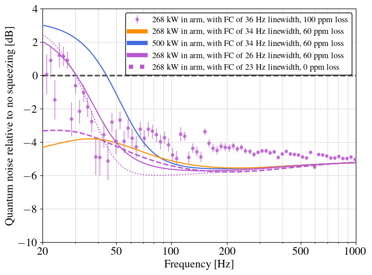
SQZ BLRMS
# %%
import numpy as np
import matplotlib.pyplot as plt
# %matplotlib inline
from datetime import datetime as dt
from gwpy.time import tconvert
import h5py
import pandas as pd

blrms_colors = ['#EC3445','#FB761F','#FCDD30','#51BC37','#1582FD','#733294']


## Set up plot
figsize = (12,3)
plt.rc('font', **{'family':'serif','serif':['Times'], 'size':30})
plt.rc('text', usetex=True)
plt.rc('axes', **{'grid':True,'grid.which':'both'})


def setup_plot(ax1, legend_title='', columnspacing=0, labelspacing=0,
               xlabel="Time [days] from 24 May 2023", xlims=(0,370),
               ylabel="SQZ [dB]", ylims=(-6,-1),
               ):
    legend = ax1.legend(loc=[-0.13,1.1], title=legend_title, ncol=6, edgecolor='black', fontsize=25,
                        title_fontsize=35,
                        columnspacing=columnspacing, handletextpad=0, markerscale=2, numpoints=1,
                        labelspacing=labelspacing, borderpad=0.3,)
    legend._legend_box.sep = 10
    ax1.minorticks_on()

    ax1.grid(True,which='both',lw=0.5,ls='-',alpha=0.5,)
    ax1.grid(which='minor',lw=0.3,ls=':',alpha=0.5,)

    ax1.set_xlabel(xlabel, labelpad=15, fontsize=30)
    ax1.set_xticks(np.arange(0,370,50))  ; ax1.set_xlim(xlims)

    ax1.set_ylabel(ylabel, labelpad=13, fontsize=30)
    ax1.set_yticks([-6,-5,-4,-3,-2,-1,]) ; ax1.set_ylim(ylims)


## Function to get sqz blrms data, when sqz bdiv is open
def get_h5_sqz_blrms_data(fname_sqz_blrms_o4):
    ''' Example usage like this:

    fname_sqz_blrms_o4 = "h1_o4_sqz_blrms"
    sqzblrms_dict = get_h5_sqz_blrms_data('data_dir'+fname_sqz_blrms_o4)
    plt.plot(sqzblrms_dict['H1:SQZ-DCPD_RATIO_5_DB_MON']['means'][::snkip],
             alpha=0.05, ls='', marker='o')
    plt.ylim(-10,20)
    '''

    # read hdf5 file
    h5 = h5py.File('../data/sqz_blrms_trends/'+fname_sqz_blrms_o4+'.hdf5','r')

    # mask data that has bdiv open
    select_on_mask = False
    for key in h5.keys():
        if 'SYS-MOTION_C_BDIV_E_POSITION' in key:
            mask = np.nan_to_num(np.array(h5[key]['max']))
            mask = np.array(mask,dtype=bool)
            select_on_mask = True
            print('selecting only data with beam diverter open')
        # if 'SQZ-GRD' in key:
        #     grd_state = np.nan_to_num(np.array(h5[key]['max']))
        #     mask = np.array(grd_state=10,dtype=bool)
        #     select_on_mask = True
        #     print('selecting only data with beam diverter open')
    if not select_on_mask:
        print('failed to select only data with beam diverter open')

    # make data into dictionary
    sqzblrms_dict={}
    for key in h5.keys():
        if 'SYS-MOTION_C_BDIV_E_POSITION' in key: continue
        print(key)

        sqzblrms_dict[key] = {}
        means = np.array(h5[key]['mean']) ; print(np.nanmedian(means))
        tts = np.arange(0,60*len(means+1),60)
        # dt = 60 # ndscope had minute trends (1 datapoint every tt=60 seconds)

        if select_on_mask:  means[mask] = np.nan ; print(f'after removing bdiv closed, {np.nanmedian(means)}')

        sqzblrms_dict[key].update(tts=tts,means=means)

    # close hdf5
    h5.close()

    return sqzblrms_dict


# %% --------  H1  ---------------------------------------------
# # H1 - Plot histogram and timeseries of kHz squeezing in days

# %%
fname_sqz_blrms_o4 = "h1_o4_blrms"

sqzblrms_dict = get_h5_sqz_blrms_data(fname_sqz_blrms_o4)

t0_gps = 1368975618 # start of ndscope ~ start of O4a 1368975618
t0_dt  = tconvert(t0_gps)


## resample data time-wise
blrms_chan = "H1:SQZ-DCPD_RATIO_5_DB_MON"
df_full = pd.DataFrame({
    'datetime': sqzblrms_dict[blrms_chan]['tts']/(60*60*24), #days,
    'blrms'   : sqzblrms_dict[blrms_chan]['means'],
})
df_full.datetime = pd.to_datetime(df_full.datetime, origin=t0_dt, unit='D')
df_full.set_index('datetime', inplace=True)

df = df_full.resample('3H',).median()

# df.reset_index().plot.scatter(x='datetime', y='blrms', rot=45)
tts   = (df.index - df.index[0]).astype(int).to_numpy()/1e9 /(60*60*24)
blrms = df['blrms'].to_numpy()


## prep plot
t0 = t0_gps # 21.5*7 # O4a started May 24 2023 1500 UTC, week 21.5
t1 = int(tconvert(dt(2023,  6, 21, 15, 0)) - t0_gps)/60/60/24  # June 20/21
t2 = int(tconvert(dt(2023, 10, 17, 15, 0)) - t0_gps)/60/60/24  # ~Oct 17 2023
t3 = int(tconvert(dt(2023, 12, 19,  0, 0)) - t0_gps)/60/60/24  # ~Dec 19 2023
t4 = int(tconvert(dt(2024,  1, 16, 16, 0)) - t0_gps)/60/60/24  # O4a ended (datetime(2024,1,16,16,0,0))
t5 = int(tconvert(dt(2024,  4, 10, 15, 0)) - t0_gps)/60/60/24  # O4b started 15:00 UTC, 10 April 2024

# get indicies for different time periods
tts1 = (tts<t1)
tts2 = (tts>t1) & (tts<t2)
tts3 = (tts>t2) & (tts<t3)
tts4 = (tts>t3) & (tts<t4)
tts5 = (tts>t4)
# tts5 = (tts>t4) & (tts<t5)
# tts6 = (tts>t5)
tts_segments = [tts1, tts2, tts3, tts4, tts5]

labels = ['72 W',
          '57 W',
          'Crystal move', #'O4a, Less crystal loss',
          'Worse matching',
          'New OMC + better matching',]

plot_colors  = [blrms_colors[1],blrms_colors[4],
                blrms_colors[0],blrms_colors[2],
                blrms_colors[5], blrms_colors[2],]

alphas  = [0.9, 0.9, 0.8, 0.8, 0.9, 0.9]
zorders = [  10,   2,   4,   6,   3,   10]
nbins = [90, 100, 200, 100, 100]

## Plot timeseries kHz squeezing
fig_h1, (ax1,ax2) = plt.subplots(figsize=figsize, ncols=2, nrows=1, sharey=True,
                         gridspec_kw={'width_ratios': [4, 1]})

plt.subplots_adjust(wspace=0.015, hspace=0, left=0, right=1, bottom=0, top=1,)
for tts_segment, blrms_color, label, zorder, alpha, nbin in zip(tts_segments,plot_colors,labels,zorders,alphas,nbins):
    yys = blrms[tts_segment]
    if 'OMC' in label: yys[yys > np.random.rand(1)*-2] = 1
    # timeseries kHz squeezing
    ax1.plot(tts[tts_segment], yys, label=label,
             color=blrms_color, alpha=0.6, ls='', marker='o', ms=5)

    # histogram plot
    ax2.hist(yys, bins=nbin, label=label, zorder=zorder,
             color=blrms_color, alpha=alpha, orientation="horizontal", )


median_lho = np.nanmedian(blrms[(tts>t2) & (blrms<-3)])
print()
print(f'median LHO sqz after crytal move ~ {median_lho} dB')
print()
print(f'median LHO sqz incl all 60W ~ {np.nanmedian(blrms[(tts>t1) & (blrms<-3)])} dB')

# timeseries kHz squeezing
setup_plot(ax1, legend_title='LHO', columnspacing=0)

# histogram
setup_plot(ax2, xlabel="", ylabel="",xlims=(0,65))
ax2.set_yticks([-6,-5,-4,-3,-2,-1,])
ax2.set(xticklabels=[], xlabel="")
ax2.get_legend().remove()


# %% --------  L1  ---------------------------------------------
print()
fname_sqz_blrms_o4 = "l1_o4_blrms"
sqzblrms_dict = get_h5_sqz_blrms_data(fname_sqz_blrms_o4)


## resample data time-wise
blrms_chan = "L1:SQZ-DCPD_RATIO_4_DB_MON"
df_full = pd.DataFrame({
    'datetime': sqzblrms_dict[blrms_chan]['tts']/(60*60*24), #days,
    'blrms'   : sqzblrms_dict[blrms_chan]['means'],
})
df_full.datetime = pd.to_datetime(df_full.datetime, origin=t0_dt, unit='D')
df_full.set_index('datetime', inplace=True)

df = df_full.resample('3H',).median()

tts   = (df.index - df.index[0]).astype(int).to_numpy()/1e9 /(60*60*24)
blrms = df['blrms'].to_numpy()


### Label major time markers in timeseries

t0 = t0_gps # 21.5*7 # O4a started May 24 2023 1500 UTC, week 21.5
t1 = int(tconvert(dt(2023,  6, 20, 12, 0)) - t0_gps)/60/60/24  # June 20/21
# t2 = int(tconvert(dt(2023,  7, 31, 15, 0)) - t0_gps)/60/60/24  # July 31 2023, LLO:66502, OMC_3Q back to CLF_6I'
t2 = int(tconvert(dt(2023, 10,  3,  0, 0)) - t0_gps)/60/60/24  # Oct 3 2023, LLO:67569, crystal move
t3 = int(tconvert(dt(2023, 11,  2,  0, 0)) - t0_gps)/60/60/24  # Nov 2 2023, LLO:68097, alignment shift
t4 = int(tconvert(dt(2024,  1, 16, 16, 0)) - t0_gps)/60/60/24  # O4a ended (datetime(2024,1,16,16,0,0))
t5 = int(tconvert(dt(2024,  4, 10, 15, 0)) - t0_gps)/60/60/24  # O4b started 15:00 UTC, 10 April 2024


# get indicies for different time periods
tts1 = (tts<t1)
tts2 = (tts>t1) & (tts<t2)
tts3 = (tts>t2) & (tts<t4)
# tts4 = (tts>t3) & (tts<t4)
tts5 = (tts>t4) #& (tts<t5)
# tts6 = (tts>t5)
tts_segments = [tts1, tts2, tts3, #tts4,
                tts5, #tts6
                ]


# labels = ['O4a Start', # start O4a
#           'June 20 2023, LLO:65737, alignment script',
#           #'July 31 2023, LLO:66502, OMC_3Q back to CLF_6I', # what happened here?
#           'Oct 3 2023,   LLO:67569, crystal move',
#           'Nov 2 2023,   LLO:68097, alignment shift',
#           'Nov 9 2023,   LLO:68211, opo temp adjust',
#           'O4b',
#          ]
labels = ['63 W',   # start O4a
          'Re-optimized alignment and matching', # June 20 2023, LLO:65737
          'Crystal move',       # Oct 3 2023, LLO:67569
          # 'O4a, Alignment shift',  # Nov 2 2023, LLO:68097
          'Re-optimized',
          'Re-optimized',
         ]

plot_colors  = [blrms_colors[1], blrms_colors[4],
                blrms_colors[0], #blrms_colors[3],
                # blrms_colors[2],
                blrms_colors[5], ]

zorders = [  7,   3,   4,   5,   1,  ]

## Plot timeseries kHz squeezing
fig_l1, (ax1,ax2) = plt.subplots(figsize=figsize, ncols=2, nrows=1, sharey=True,
                         gridspec_kw={'width_ratios': [4, 1]})
plt.subplots_adjust(wspace=0.015, hspace=0, left=0, right=1, bottom=0, top=1,)

for tts_segment, blrms_color, label, zorder in zip(tts_segments,plot_colors,labels,zorders):

    # timeseries kHz squeezing
    ax1.plot(tts[tts_segment], blrms[tts_segment], label=label,
             color=blrms_color, alpha=0.6, ls='', marker='o', ms=5)

    # histogram plot
    ax2.hist(blrms[tts_segment], bins=200, label=label, zorder=zorder,
             color=blrms_color, alpha=0.9, orientation="horizontal", )


median_llo = np.nanmedian(blrms)
print()
print(f'median LLO sqz ~ {median_llo} dB')

# timeseries kHz squeezing
setup_plot(ax1, legend_title='LLO', columnspacing=0.4)

# histogram
setup_plot(ax2, xlabel="", ylabel="",xlims=(0,85))
ax2.set_yticks([-6,-5,-4,-3,-2,-1,])
ax2.set(xticklabels=[], xlabel="")
ax2.get_legend().remove()


# %%  save data and figures
# fig_l1.set_size_inches(6,3)
fig_l1.savefig(fname_sqz_blrms_o4+'_2kHz_blrms_by_config.pdf',bbox_inches='tight')


# fig_h1.set_size_inches(6,3)
fname_sqz_blrms_o4 = "h1_o4_blrms"
fig_h1.axes[0].axes.xaxis.set_ticklabels([])
fig_h1.axes[0].axes.set_xlabel(None)
fig_h1.savefig(fname_sqz_blrms_o4+'_2kHz_blrms_by_config.pdf',bbox_inches='tight')


plt.show()
selecting only data with beam diverter open
H1:SQZ-DCPD_RATIO_5_DB_MON
-3.2653167163332304
after removing bdiv closed, -3.6443573478609324

median LHO sqz after crytal move ~ -4.044899665067593 dB

median LHO sqz incl all 60W ~ -3.730494447549184 dB

selecting only data with beam diverter open
L1:SQZ-DCPD_RATIO_4_DB_MON
-4.667612255116304
after removing bdiv closed, -5.106696502367655

median LLO sqz ~ -5.084431870778402 dB
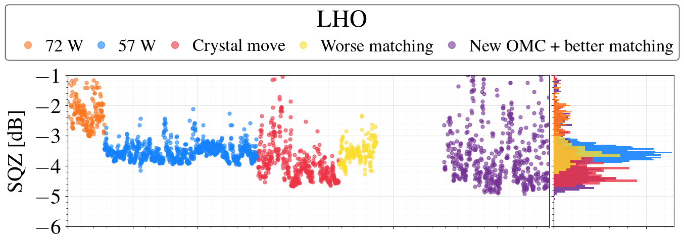
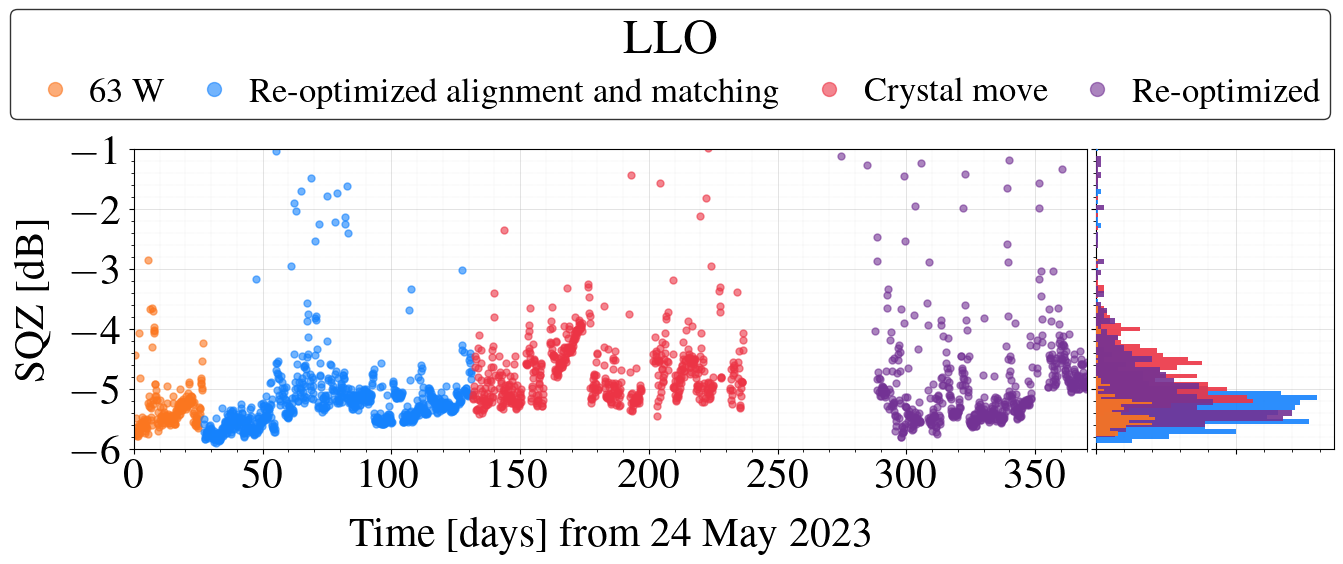
# save HDF5 darm traces to txt files for easier later

# np.savetxt('../data/noise_budget/L1_O4_strain_asd_withSqueezing.txt',
#            np.c_[l1nb['Freq'][:], np.sqrt(l1nb['L1/budget/DARMMeasured/PSD'][:]/L_arm**2)],
#            fmt='%.15e', header='L1, O4a, frequency [Hz], strain asd [1/rtHz]')

# np.savetxt('../data/noise_budget/lho_darm_noisebudget_O4a_hotOM2_start1386255618_span1800.txt',
#            np.c_[h1nb['Freq'][:], np.sqrt(h1nb['H1/budget/DARMMeasured/PSD'][:]/L_arm**2)],
#            fmt='%.15e', header='H1, O4a, frequency [Hz], strain asd [1/rtHz]')

# np.savetxt('../data/noise_budget/lho_correlated_darm_noisebudget_start1386718819_span900.txt',
#            np.c_[h1nb_xcorr['Freq'][:], np.sqrt(h1nb_xcorr['CorrelatedDARM/budget/DARMMeasured/PSD'][:]/L_arm**2)],
#            fmt='%.15e', header='H1, O4a, frequency [Hz], unsqz strain asd [1/rtHz]')